Influences on the Supply of Labour to Markets (AQA A-Level Economics): Revision Notes
Influences on the Supply of Labour to Markets
Introduction to the market supply of labour
The market supply of labour shows the total quantity of labour that all workers in a particular labour market are willing to supply at different wage rates. Just as firms have supply curves for their products, workers have a supply curve for the labour they provide. This supply curve is fundamental to understanding how labour markets operate and how wages are determined.
When we talk about labour supply, we're referring to the number of hours workers are prepared to work in a given time period (such as per week or per year). This supply depends on many factors, with the wage rate being the most obvious, but also including various non-monetary considerations that affect workers' decisions.
The market supply of labour curve
The market supply curve of labour typically slopes upward from left to right, showing a positive relationship between wage rates and the quantity of labour supplied. This means that as hourly wage rates increase, workers are generally willing to supply more hours of labour to the market.
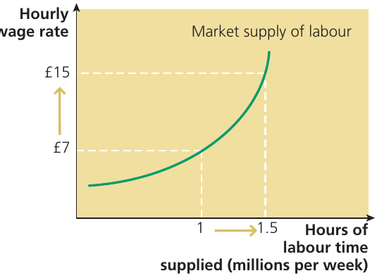
The graph illustrates how workers respond to wage changes. For example, when the hourly wage rate increases from $7 to $15, workers increase the total number of hours they're prepared to work from 1 million to 1.5 million hours per week. This upward slope reflects the fundamental economic principle that higher rewards encourage more supply.
However, it's important to understand that this relationship isn't always straightforward. Workers must balance their desire for income against their need for leisure time, and this creates interesting dynamics in labour supply decisions.
Monetary and non-monetary considerations
The role of the money wage rate
The money wage rate (the actual hourly or weekly pay received) is the primary factor influencing how much labour workers are willing to supply. For most people, both the wage received and the time available for leisure are important because of the economic principle of diminishing marginal utility. This means that as we consume more of something, each additional unit provides less satisfaction than the previous one.
Higher wages provide a monetary incentive for workers to supply more labour. The additional income allows workers to purchase more goods and services, increasing their material standard of living. This is why the supply curve generally slopes upward - people are willing to work more hours when the financial reward is greater.
Non-monetary benefits and job satisfaction
Beyond the wage, workers also consider non-monetary benefits when deciding how much labour to supply. These non-monetary considerations (sometimes called non-pecuniary benefits) include factors such as:
- Job satisfaction or dissatisfaction from the work itself
- Working conditions and environment
- Job security
- Promotion prospects and career development
- Holiday entitlement
- Psychological benefits or stress from the work
When a worker enjoys their job, the overall benefit of working (called the net advantage) is greater than the wage alone. In this situation, a worker might be willing to accept a lower wage than they would demand for unpleasant work. Conversely, unpleasant or dangerous work - such as routine assembly-line tasks or heavy manual labour - requires higher wages to compensate for the job dissatisfaction it causes.
The work-leisure trade-off
Workers face a fundamental choice about how to allocate their 24 hours each day. They must decide between supplying more labour (which earns income to buy goods and services) and enjoying more leisure time (which provides direct satisfaction but no income).
This decision involves weighing up the benefits of earning additional income against the cost of sacrificing leisure time. As workers supply more labour hours at a particular wage rate, they earn extra income but also experience less satisfaction from each additional hour worked, because they have less leisure time remaining. The opportunity cost of working one more hour is the leisure time that must be given up.
Finding the optimal balance
Workers aim to maximise their overall welfare (called net advantage) by finding the right balance between work and leisure. At the optimal point, the satisfaction gained from the last unit of income earned equals the satisfaction lost from giving up the last unit of leisure time. We can express this as:
At this point, the marginal private benefit (additional income and its purchasing power) equals the marginal private cost (leisure time foregone). If the wage rate stays the same and a worker is already at this optimal balance, there's no incentive to supply more labour.
Understanding the Upward-Sloping Supply Curve
When wages rise, the situation changes. A higher hourly wage means that the welfare gained from earning money becomes greater than the welfare lost from sacrificing the last unit of leisure. To maximise their overall welfare at this higher wage rate, workers will choose to supply more labour hours and enjoy less leisure time. This explains why the labour supply curve slopes upward - higher wages encourage workers to work more hours.
It's worth noting that individual workers' job choices depend on both the money wage rate and the job satisfaction they expect to derive from different occupations. While non-monetary factors usually change slowly, a rise in wages in a particular occupation typically leads to an increase in the supply of labour to that occupation.
Shifts of the market supply curve of labour
While changes in wage rates cause movements along the supply curve, other factors can shift the entire supply curve to a new position. These shifts mean that at every wage rate, workers are willing to supply either more labour (rightward shift) or less labour (leftward shift).
Changes in non-monetary factors
Improvements in non-monetary benefits shift the supply curve of labour to the right, meaning workers are willing to supply more labour at each wage rate. These factors include:
- Job security: Greater job security makes positions more attractive
- Promotion prospects: Better career advancement opportunities increase labour supply
- Working conditions: Improved workplace environments and better conditions attract more workers
- Holiday entitlement: More generous holiday allowances make jobs more appealing
- Psychological benefits: Work that provides greater satisfaction or purpose increases supply
Conversely, a deterioration in these non-monetary benefits shifts the supply curve to the left. Workers become less willing to supply labour at each wage rate because the overall attractiveness of the work has decreased.
The Leisure Preference Principle
If people decide they value leisure more highly, they will work fewer hours at each wage rate, and the supply curve shifts left. If they decide they want more goods and services rather than leisure time, the supply curve shifts to the right.
Changes in income
Changes in workers' income levels can affect labour supply, though the direction of the effect depends on whether leisure is considered a normal good or an inferior good for that worker.
For most people, leisure time is a normal good. This means that as income rises, people demand more leisure (and therefore supply less labour). A rise in income increases the demand for leisure time, which causes the supply curve of labour to shift to the left. Workers with higher incomes may choose to work fewer hours and enjoy more leisure time instead.
However, for some individuals, leisure might be an inferior good. These people prefer to spend their higher income on more goods and services rather than leisure time. For them, higher income reduces their demand for leisure and causes them to supply more labour. This shifts the supply curve to the right.
Changes in population
Population changes have significant effects on labour supply:
- Rising population: An increase in population, perhaps caused by immigration, increases the supply of labour. More people of working age mean more potential workers, shifting the supply curve to the right.
- Falling population: A reduction in the number of working-age people causes the labour supply curve to shift to the left.
- Retirement age changes: A fall in the number of people of working age (for example, due to many workers reaching retirement age) shifts the supply curve to the left. However, this effect can be offset if older workers decide to work longer to finance their eventual retirement.
These population effects are particularly important for understanding long-term trends in labour markets and why governments often focus on immigration policy and retirement age regulations.
Changes in expectations
Workers' expectations about the future can also shift the labour supply curve:
- Pension expectations: If older people expect to live longer but become less optimistic about their future pension incomes, they may increase their labour supply. This causes the supply curve to shift to the right as workers seek to earn more to secure their retirement.
- Education trends: A rise in the proportion of people staying in further and higher education tends to reduce the supply of labour in the short term, shifting the supply curve to the left. Students are not supplying labour during their study years, though their education may increase their productivity and labour supply in the long term.
Understanding these expectation effects helps explain changing patterns in labour market participation across different age groups and education levels.
The elasticity of supply of labour
Definition and measurement
Elasticity of supply of labour measures how responsive the quantity of labour supplied is to a change in the wage rate. It's calculated using the following formula:
This concept is crucial for understanding how labour markets respond to wage changes. Some labour markets are very responsive to wage increases (elastic supply), while others show little response (inelastic supply).
Factors determining the elasticity of supply of labour
Several key factors influence how elastic the supply of labour is in a particular market:
Skilled versus unskilled labour: The supply of unskilled labour is usually more elastic than the supply of skilled labour. This is because the training period for unskilled work is typically very short, and the innate abilities required are common among the population. Anyone can relatively quickly become an unskilled worker. In contrast, skilled labour requires longer training periods and may require specific aptitudes that only a limited proportion of the population possesses, making supply less responsive to wage changes.
Understanding Labour Mobility
Factors that reduce workers' ability to move between occupations or locations tend to reduce the elasticity of labour supply. Occupational mobility refers to how easily workers can change professions - this depends on whether they can acquire the necessary skills and qualifications. Geographical mobility relates to how easily workers can move to where jobs are located. When workers face barriers to either type of mobility (such as family commitments, housing costs, or qualification requirements), the supply of labour becomes more inelastic.
Time period: The supply of labour is more elastic in the long run than in the short run. Over longer time periods, workers have more opportunity to retrain, relocate, or adjust their work-leisure preferences in response to wage changes. In the short run, workers are more constrained in their ability to respond to wage changes.
Unemployment levels: The availability of a pool of unemployed workers increases the elasticity of supply of labour. When unemployment is high, there are more potential workers who can quickly enter the labour market when wages rise. Conversely, when there is full employment, supply is more inelastic because there are fewer available workers to recruit.
Worked example: calculating wage elasticity of supply
Worked Example: Calculating Wage Elasticity of Supply
Scenario: A firm facing a labour shortage increases the wage it pays from $10 per hour to $15 per hour. As a result, the number of workers applying for jobs at the firm increases from 1,000 to 1,500 workers.
Question: What is the wage elasticity of supply of labour with respect to this wage rate increase?
Solution:
Step 1: Calculate the percentage change in quantity of labour supplied:
- Change in quantity = 1,500 - 1,000 = 500 workers
- Percentage change =
Step 2: Calculate the percentage change in wage rate:
- Change in wage = $15 - $10 = $5
- Percentage change =
Step 3: Apply the formula:
Interpretation: The wage elasticity of supply is equal to 1 (unitary elasticity). This means that the percentage change in labour supplied exactly matches the percentage change in the wage rate. For every 1% increase in wages, there is a 1% increase in labour supplied.
This calculation demonstrates that between these two wage rates, labour supply is neither particularly elastic nor inelastic - it shows a proportionate response to the wage change.
Remember!
Key Points to Remember:
-
The market supply of labour curve shows the total quantity of labour workers are willing to supply at different wage rates, typically sloping upward as higher wages encourage more work.
-
Workers consider both monetary factors (the wage rate) and non-monetary factors (such as job satisfaction, working conditions, and job security) when deciding how much labour to supply.
-
The work-leisure trade-off is fundamental: workers must balance their desire for income against their need for leisure time, with the opportunity cost of working being the leisure time sacrificed.
-
Various factors can shift the entire supply curve, including changes in non-monetary benefits, income levels, population size, and worker expectations about the future.
-
Elasticity of supply of labour measures responsiveness to wage changes and depends on factors such as skill level, worker mobility, the time period considered, and unemployment levels.