Chi-Square Test (AQA A-Level Geography): Revision Notes
Chi-Square Test
What is the chi-square test?
The chi-square test (written as χ²) is a statistical technique that helps you determine whether differences between observed and expected data are genuine patterns or simply due to chance. This test is particularly useful in geographical fieldwork when you want to compare real-world data you've collected with what theory predicts should happen.
The test works by comparing two sets of data:
- Observed data (O): The actual measurements or counts you've collected during fieldwork or obtained from secondary sources
- Expected data (E): The theoretical values you would expect to find if there were no pattern or if a particular theory were correct
The chi-square test produces a numerical value that you can then compare against standard statistical tables to assess whether any pattern in your data is statistically significant. This comparison allows you to make objective decisions about your data rather than relying on subjective interpretation.
Understanding the components
Observed and expected data
When conducting a chi-square test, you're essentially asking: "Does my real-world data match what I expected to find?"
Observed data represents what you've actually measured or counted in the field. For example, if you're studying beach pebble orientations, the observed data would be the actual number of pebbles pointing in each direction.
Expected data represents what you would anticipate finding based on a theoretical assumption. If pebbles were randomly oriented with no preferred direction, you would expect equal numbers pointing in all directions. This becomes your expected distribution.
Formulating a null hypothesis
Before conducting the test, you must create a null hypothesis. This is a statement that assumes there is no significant difference or relationship in your data.
Understanding the Null Hypothesis
A null hypothesis states that any pattern observed in the data is not statistically significant and could have occurred by chance. It assumes there is no real difference between the observed and expected distributions.
For example, if studying corrie orientations, your null hypothesis might state: "There is no significant difference between the observed orientation of corries and a random orientation pattern."
The alternative hypothesis (which you're actually testing for) would be that there is a significant difference, meaning some geographical factor is influencing the pattern.
The chi-square formula
The chi-square statistic is calculated using this formula:
Where:
- = the chi-square value (the Greek letter 'chi')
- = sum of (add together all the values)
- = observed frequency
- = expected frequency
This formula might look complex, but it follows a logical sequence:
- Find the difference between each observed and expected value
- Square each difference
- Divide each squared difference by the expected value
- Add all these values together to get your chi-square statistic
The formula structure can be remembered as: "O minus E, squared, over E" - this simple phrase captures the entire calculation process and helps you remember the order of operations.
Working through a calculation
Let's examine a practical example to understand how the chi-square test works in a geographical context.
Worked Example: Corrie Orientations in Snowdonia
A group of students investigated whether corries (circular hollows carved by ice) in Snowdonia showed a preferred orientation. They measured 40 corries and categorised them into four directional groups based on the direction they faced.
The students wanted to determine if the corries faced particular directions (perhaps due to prevailing wind or sunlight patterns) or if their orientation was random.
Their null hypothesis was: "There is no significant difference between the observed orientation of the corries and expected random orientation."
Step-by-step calculation process:
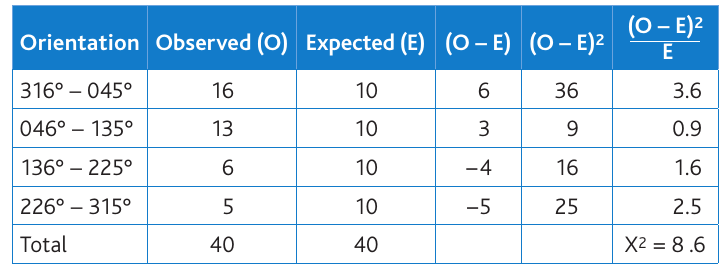
Step 1: Record observed values (O)
Lists the actual number of corries found facing each direction:
- 16 corries faced between 316°-045° (roughly north)
- 13 corries faced between 046°-135° (roughly east)
- 6 corries faced between 136°-225° (roughly south)
- 5 corries faced between 226°-315° (roughly west)
- Total = 40 corries
Step 2: Calculate expected values (E)
Shows the number expected if corries were randomly oriented. Since there are four equal directional categories and 40 corries total, we expect 10 corries in each direction .
Step 3: Find the difference (O-E)
Calculate the difference between observed and expected for each category:
- 316°-045°:
- 046°-135°:
- 136°-225°:
- 226°-315°:
Step 4: Square each difference (O-E)²
Square each difference to eliminate negative values:
Step 5: Divide by expected value (O-E)²/E
Divide each squared difference by the expected value:
Step 6: Sum all values
Add all the values in the final column:
The calculated chi-square value is
Calculating degrees of freedom
Before you can interpret your chi-square value, you need to work out the degrees of freedom. This is a statistical concept that relates to the number of categories in your data.
The formula is simple:
Where is the number of categories (or cells) containing observed data.
Calculating Degrees of Freedom for the Corrie Example:
- There are 4 directional categories
- Degrees of freedom =
This value is essential because you'll need it to look up the correct critical value in statistical tables. Think of it as "Freedom = n minus 1" - a simple way to remember the calculation.
Interpreting your results
Using critical values
Once you've calculated your chi-square value and degrees of freedom, you need to determine whether your result is statistically significant. This is done by comparing your calculated value against critical values in a standard statistical table.
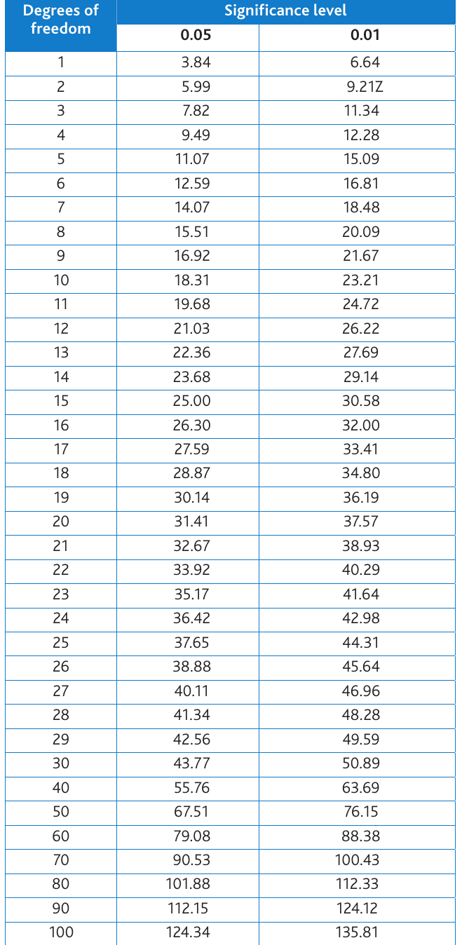
The critical values table shows the minimum chi-square value needed for significance at different degrees of freedom and significance levels.
Significance levels
There are two standard significance levels used in geographical studies:
-
0.05 significance level (95% confidence): There is only a 5% (1 in 20) probability that the pattern occurred by chance. This means you can be 95% confident that the pattern is real.
-
0.01 significance level (99% confidence): There is only a 1% (1 in 100) probability that the pattern occurred by chance. This means you can be 99% confident that the pattern is real.
These are also called confidence levels. Higher confidence levels provide stronger evidence that your results are genuine and not due to random chance. The standard levels of 95% and 99% are widely accepted in geographical research.
Making your decision
To interpret your results, follow these steps:
- Look up your degrees of freedom in the left column of the critical values table
- Read across to find the critical values at both significance levels
- Compare your calculated chi-square value to these critical values
Decision rules:
-
If your calculated value is equal to or greater than the critical value: You can reject the null hypothesis. This means the difference between observed and expected data is statistically significant.
-
If your calculated value is less than the critical value: You must accept the null hypothesis. This means any pattern in your data could have occurred by chance.
Remember: "Big chi means reject" - if your calculated is larger than the critical value, you reject the null hypothesis and conclude there is a significant pattern in your data.
Applying this to the corrie example
In the corrie orientation study:
- Calculated value = 8.6
- Degrees of freedom = 3
- Critical value at 0.05 level (3 degrees of freedom) = 7.82
- Critical value at 0.01 level (3 degrees of freedom) = 11.34
The calculated value (8.6) is greater than 7.82 but less than 11.34. This means:
- The result IS significant at the 0.05 (95%) level
- The result IS NOT significant at the 0.01 (99%) level
Therefore, the null hypothesis can be rejected at the 95% confidence level. The students can conclude with 95% confidence that corries in Snowdonia do show a preferred orientation rather than being randomly oriented.
Important considerations and limitations
When using the chi-square test in your geographical investigations, you must keep several important points in mind:
Sample size requirements
Minimum Sample Size Requirement
Both your observed and expected values must be large enough for the test to be valid. Most statisticians recommend a minimum of five observations per category. If your categories contain fewer than five observations, the test results may not be reliable and your conclusions could be flawed.
The meaning of the chi-square value
The number you calculate is only meaningful when compared to critical values in statistical tables. The chi-square value itself (such as 8.6 in our example) doesn't directly tell you anything - it must be interpreted using the table.
Appropriate application
You should not apply the chi-square test to more than one set of observed data because the mathematical calculations become too complex and unreliable.
Supporting geographical understanding
Using Statistics to Support Geography
The chi-square test should support your geographical thinking, not replace it. Use it to strengthen your arguments and test your hypotheses, but always:
- Relate your statistical results back to geographical theory
- Consider what geographical processes might explain significant patterns
- Acknowledge when results don't match expectations and explore why
- Use the test as evidence within broader geographical analysis
If your results support your hypothesis, excellent - you have statistical evidence for your ideas. If your results contradict your hypothesis, this is equally valuable as it may indicate unexpected geographical factors at work or suggest areas for further investigation.
Making geographical sense
Above all, your investigation should make geographical sense. Demonstrating statistical ability is less important than showing you understand the geographical significance of your findings. Always explain what your results mean in terms of geographical processes, patterns and theories.
Key Points to Remember:
-
The chi-square test compares observed data from fieldwork with expected data from theory to determine if differences are statistically significant or due to chance
-
Calculate chi-square using the formula: , which involves finding differences, squaring them, dividing by expected values, and summing the results
-
Degrees of freedom = , where is the number of categories containing data - you need this to use the critical values table
-
Compare your calculated value against critical values at either 95% (0.05) or 99% (0.01) confidence levels - if your value is equal to or greater, reject the null hypothesis
-
Always ensure your sample sizes are adequate (minimum 5 per category), relate your results to geographical theory, and prioritise geographical understanding over mathematical complexity