Spearman Rank Correlation Coefficient (AQA A-Level Geography): Revision Notes
Spearman Rank Correlation Coefficient
What is the Spearman rank correlation coefficient?
The Spearman rank correlation coefficient is a statistical test that measures the strength and direction of correlation between two sets of data (also called variables). It tells us whether there is a relationship between two variables and how strong that relationship is.
This test provides a numerical value that summarises the degree of correlation. It is an objective indicator, meaning the result can be tested statistically to see how meaningful it is. Once you calculate the coefficient, you must test it against critical values to determine whether the result is significant or could have occurred by chance.
Correlation vs. Causation
Correlation between two variables does not prove a causal link. Even if there is a relationship between altitude and precipitation, for example, a decrease in one does not automatically cause a decrease in the other. They are simply related to each other. The relationship does not prove that a change in one variable is responsible for a change in the other.
When to use this test
The Spearman rank correlation coefficient can be used with:
- Raw numerical figures
- Percentages
- Index values
- Any data that can be ranked in order
The key requirement is that your data must be capable of being ranked from highest to lowest (or vice versa).
The formula
The Spearman rank correlation coefficient uses the following formula:
Where:
- = the Spearman rank correlation coefficient
- = the difference in ranking between the two sets of paired data
- = the number of sets of paired data
- = sum of (add together all values)
Step-by-step calculation method
Follow these steps carefully to calculate the Spearman rank correlation coefficient:
Step 1: Rank the first data set
Rank one set of data from highest to lowest. The highest value receives rank 1, the second highest receives rank 2, and so on.
Step 2: Rank the second data set
Rank the other set of data in exactly the same way (highest to lowest).
Step 3: Deal with tied ranks
If you have tied values (numbers that are the same), you need to allocate an average rank:
Handling Tied Ranks
For example, if three values should all be placed at rank 5:
- Add together the ranks 5, 6 and 7
- Divide by three
- This gives an average rank of 6 for each of those three values
- The next value in the sequence would then be allocated rank 8
Step 4: Calculate the difference in ranks
For each pair of data, calculate the difference between the two ranks. This is your value.
Step 5: Square each difference
Square each value to get .
Step 6: Add the squared differences
Add all the values together. This gives you (the sum of squared differences).
Step 7: Multiply by 6
Multiply your value by 6. This gives you the numerator: .
Step 8: Calculate n³ - n
Calculate the value of , where is the number of pairs of data. This is your denominator.
Step 9: Divide and subtract from 1
Divide the result from Step 7 by the result from Step 8, then take this answer away from 1.
The final answer should be a value between +1.0 (perfect positive correlation) and -1.0 (perfect negative correlation).
Worked example
Let's examine a study comparing the number of doctors per 1,000 population against confirmed malaria cases per 1,000 population in Asia-Pacific countries.
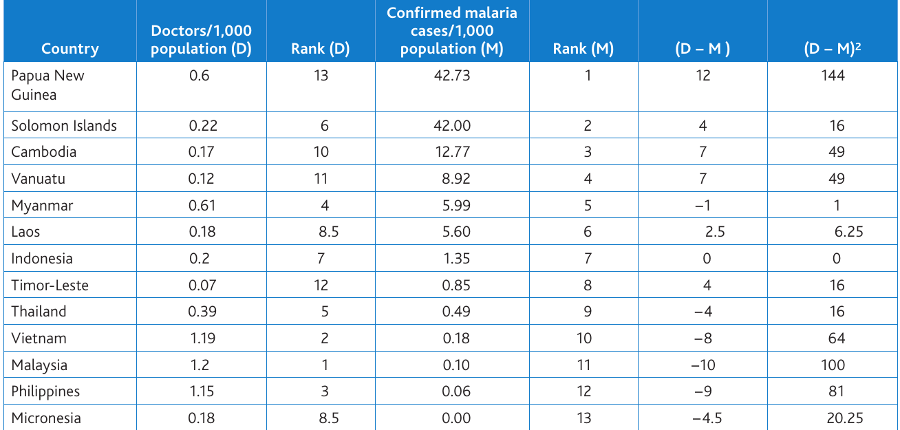
Worked Example: Doctors vs. Malaria Cases
Given data:
- Number of countries:
- Sum of squared differences:
Applying the formula:
Step-by-step calculation:
Result: The correlation coefficient is , indicating a moderate negative correlation between doctor density and malaria cases.
Second example: COVID-19 deaths and healthcare spending
Another example examines the relationship between COVID-19 deaths (up to 12 March 2020) and the percentage of GDP spent on healthcare.
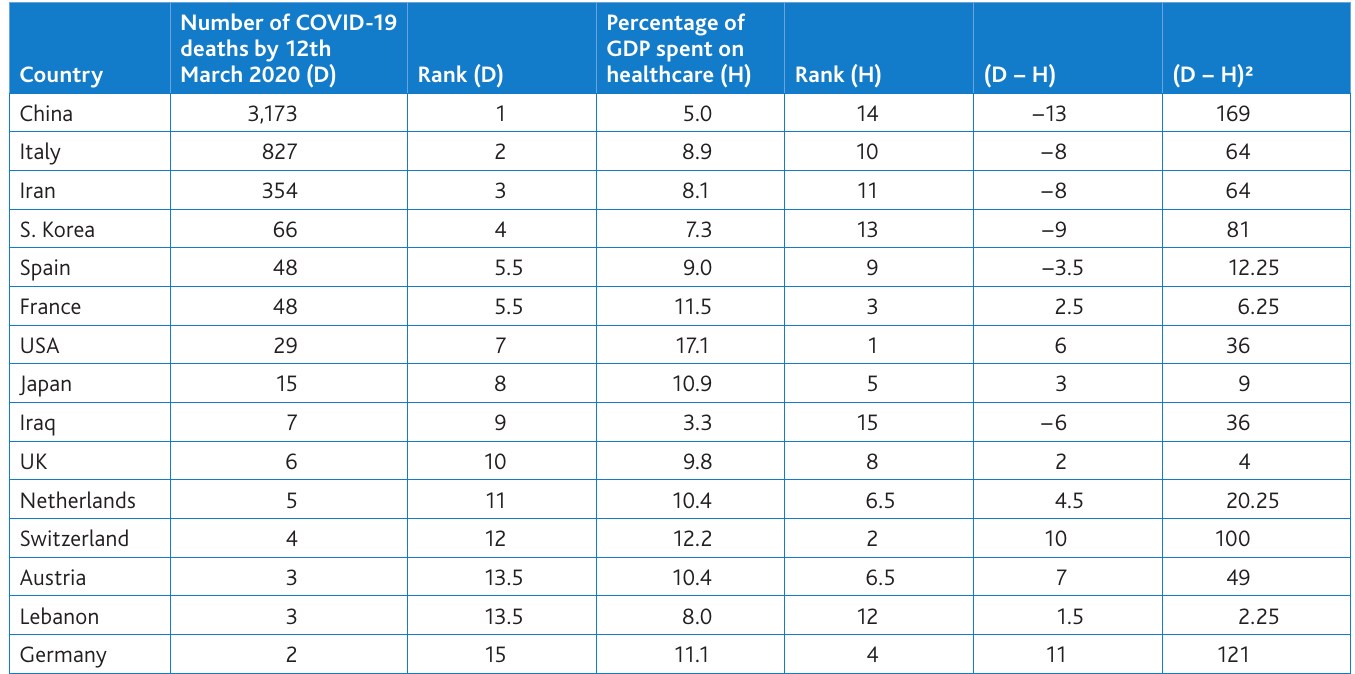
Worked Example: COVID-19 Deaths vs. Healthcare Spending
Given data:
- Number of countries:
- Sum of squared differences:
Applying the formula:
Step-by-step calculation:
Result: The correlation coefficient is , indicating a weak to moderate negative correlation between COVID-19 deaths and healthcare spending.
Interpreting your results
Direction of the relationship
The sign (positive or negative) of your coefficient tells you the direction of the relationship:
Positive correlation: If the calculation produces a positive value (e.g., ), the relationship is positive or direct. As one variable increases, so does the other.
Negative correlation: If the calculation produces a negative value (e.g., ), the relationship is negative or inverse. As one variable increases, the other decreases.
The closer the value is to or , the stronger the correlation. A value close to 0 suggests little or no correlation.
Testing for statistical significance
Simply calculating a correlation coefficient is not enough. You must test whether the relationship is statistically significant or could have occurred by chance.
Always Test for Significance
There is always a possibility that any relationship shown between two variables has occurred by chance. The numbers in the data sets may just happen to have been the right ones to produce a correlation. It is therefore necessary to assess the statistical significance of the result.
To test significance, compare your calculated value against critical values in a significance table. The critical values depend on:
- Your sample size ()
- The significance level you are testing (usually 0.05 or 0.01)
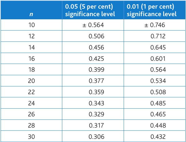
How to use the critical values table:
- Find the row for your sample size ()
- Look at the critical values for both the 0.05 (5%) and 0.01 (1%) significance levels
- Compare your calculated value with these critical values (ignore whether your value is positive or negative - just compare the absolute size)
- If your coefficient is greater than the critical value, the correlation is significant at that level
Understanding significance levels
0.05 (5%) significance level: This means there is a greater than 5% possibility of the relationship occurring by chance. If your result is significant at this level, the relationship could have occurred by chance more than 5 times in 100, which is considered an unacceptable level of chance. Therefore, the relationship is not significant.
0.01 (1%) significance level: If there is a less than 5% possibility, the relationship is significant and therefore meaningful. The stricter 0.01 (1%) level means there is less than a 1% chance the relationship occurred by chance.
Less than 1% significance: If there is less than a 1% possibility of the relationship occurring by chance, the relationship is very significant. The result could only have occurred by chance 1 in 100 times, which is very unlikely.
Applying this to our example
In the malaria example, our value was from 13 sets of paired data.
Interpreting the Malaria Example Results
Looking at Table 12.5:
- At the 0.05 (5%) level, the critical value for is 0.506
- At the 0.01 (1%) level, the critical value for is 0.712
Comparison: Since but , the relationship is significant at the 0.05 (5%) level, but not at the 0.01 (1%) level.
Conclusion: Our negative correlation between doctor density and malaria cases is statistically significant, though not at the strictest level of testing.
Important requirements and warnings
Sample size requirements
Minimum sample size: You should have at least 10 sets of paired data. The test is unreliable if .
Maximum sample size: You should have no more than 30 sets of paired data, or the calculations become too complex and prone to error.
Dealing with tied ranks
Too many tied ranks can interfere with the statistical validity of the exercise. Although it is understood that the real data collected may have tied values, there is little you can do about this. Be aware that excessive tied ranks can affect the reliability of your results.
Choosing variables carefully
Choose Variables Wisely
Be careful about choosing the variables to compare. Do not choose obviously spurious sets of data. The variables should have a logical reason to be compared, based on geographical theory or your research hypothesis.
Remember!
Key Points to Remember:
- The Spearman rank correlation coefficient measures the strength and direction of correlation between two variables
- Results range from +1.0 (perfect positive correlation) to -1.0 (perfect negative correlation)
- The formula is:
- Always test your result for statistical significance using critical values tables - don't just calculate the coefficient
- You need between 10 and 30 sets of paired data for reliable results
- Correlation does not prove causation - a relationship between variables doesn't mean one causes the other