Monopoly (Edexcel A-Level Economics A): Revision Notes
Monopoly
Introduction to monopoly
A monopoly is a market structure where there is only one seller of a good or service. This single firm has complete market power and faces no direct competition. The monopoly model helps us understand how firms behave when they have significant control over their market.
The monopoly model sits at the opposite end of the market structure spectrum from perfect competition. While perfectly competitive firms are price takers with no market power, monopolists are price makers with substantial control over market outcomes.
Key assumptions
The economic model of monopoly rests on three fundamental assumptions:
-
Single seller - There is only one firm producing and selling the good in the market.
-
No substitutes - There are no close substitutes for the product, either actual or potential. Consumers who want the product must buy from the monopolist.
-
Barriers to entry - Significant barriers to entry prevent other firms from entering the market to compete with the monopolist.
The model also assumes that the monopoly firm aims to maximise profits. These assumptions stand in sharp contrast to those of perfect competition. In fact, monopoly can be thought of as sitting at the opposite end of the market structure spectrum.
The absence of substitutes means the monopolist is protected from competition. The barriers to entry ensure this protection continues into the future, allowing the firm to sustain its market position. If potential substitutes existed, they would weaken the monopolist's market power significantly.
Monopoly in equilibrium
Understanding the monopolist's position
Unlike firms in perfect competition, a monopoly firm faces the entire market demand curve. This gives the monopolist significant influence over price. The firm is a price maker rather than a price taker, meaning it can choose different points along the demand curve by varying output levels.
However, the monopolist cannot set both price and quantity independently. The firm is still constrained by market demand. If the monopolist chooses a high price, consumers will buy less. If it wants to sell more, it must accept a lower price. The firm must choose a location along the demand curve.
For the monopolist, the market demand curve represents average revenue (AR) - the price received per unit sold. Since this demand curve slopes downwards, the monopolist faces a trade-off: selling more units requires reducing the price on all units sold.
Elasticity and total revenue
The relationship between price elasticity of demand and total revenue is crucial for understanding monopoly behaviour. This relationship determines where on the demand curve a profit-maximising monopolist will choose to operate.
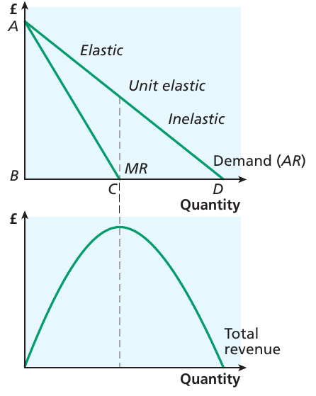
The diagram shows how price elasticity varies along a straight-line demand curve. In the upper portion, demand is price elastic - a fall in price leads to a proportionally larger increase in quantity demanded, so total revenue rises. At the midpoint of the demand curve, demand has unit elasticity - total revenue is at its maximum. In the lower portion, demand is price inelastic - a fall in price leads to a proportionally smaller increase in quantity, so total revenue falls.
Key insight for monopolists: A profit-maximising monopolist will always produce in the elastic portion of the demand curve where marginal revenue is positive. Why? Because in the inelastic range, reducing output would increase both price and total revenue while also reducing costs - clearly increasing profits.
Marginal revenue
The marginal revenue (MR) curve shows the additional revenue gained from selling one more unit of output. For a monopolist, MR lies below the demand curve (AR). This happens because to sell an additional unit, the monopolist must reduce the price not only on that extra unit but on all previous units as well.
For a straight-line demand curve, the MR curve has a special mathematical relationship with the AR curve: it shares the same vertical intercept and has exactly twice the slope. This means the MR curve cuts the horizontal axis at half the quantity where the AR curve does.
Study tip: When drawing diagrams with a downward-sloping straight-line demand curve, remember that MR and AR meet at point A (the vertical intercept), and the distance BC is the same as the distance CD. MR equals zero at the maximum point of the total revenue curve.
Profit maximisation
Like all firms, a monopolist maximises profits by producing where marginal revenue equals marginal cost (). Having determined this optimal output level, the monopolist then identifies the maximum price consumers will pay for that quantity by reading up to the demand curve.
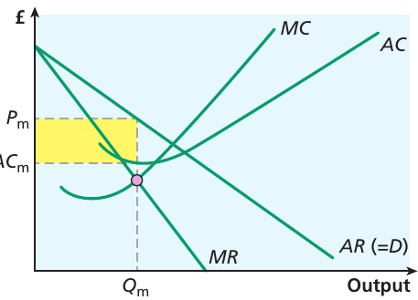
The diagram illustrates monopoly profit maximisation. The firm produces output where . At this output level, the firm charges price . The yellow shaded area represents supernormal profit - the profit above the normal return needed to keep the firm in the industry. This is calculated as:
or the profit per unit multiplied by the number of units sold.
Notice that the monopolist always produces in the segment of the demand curve where MR is positive, which is where demand is price elastic. This is because when MR is positive, the firm can increase total revenue by producing more; when MR is negative (inelastic demand), the firm would reduce total revenue by expanding output.
Barriers to entry protect profits
The existence of barriers to entry is critical for understanding why monopolists can earn supernormal profits in the long run. In a perfectly competitive market, supernormal profits attract new firms, increasing supply and pushing down prices until only normal profits remain.
However, barriers to entry prevent this competitive process from occurring in a monopoly market. Other firms cannot enter to compete away the supernormal profits. The monopolist's market position remains secure, allowing these high profits to persist indefinitely.
Without barriers to entry, a monopoly would not remain a monopoly. The assumption of no potential substitutes reinforces this protection.
Possibility of losses
A monopolist is not guaranteed to make supernormal profits. The size of profits depends on the position of the demand curve relative to the cost curves.
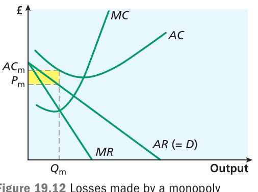
If the monopolist's costs are relatively high compared to the market demand, the firm may actually make losses in the short run. In this situation, if the firm produces where , it charges price , but this price is below average cost . The yellow area shows the loss per unit multiplied by quantity.
However, this loss-making situation cannot persist in the long run. Without the prospect of at least normal profits, the firm would eventually exit the market. This differs from the long-run equilibrium where barriers to entry protect supernormal profits.
Changes in market conditions
Response to increased demand
If a monopoly experiences (or can induce) an increase in demand for its product, the firm benefits through higher profits. When demand increases, both the demand curve (AR) and the marginal revenue curve shift to the right.
Initially, the monopoly faces demand curve and produces output at price where . When demand increases to , the MR curve shifts to (notice the fixed relationship between AR and MR). The monopolist now produces output where and charges the higher price , earning higher profits than before.
This analysis shows why monopolists may invest in advertising and marketing to shift demand rightward - doing so allows both higher prices and higher output, increasing total revenue and profits.
Response to increased costs
Suppose a monopoly experiences an increase in its average cost, perhaps caused by an increase in variable costs like wages or raw material prices.
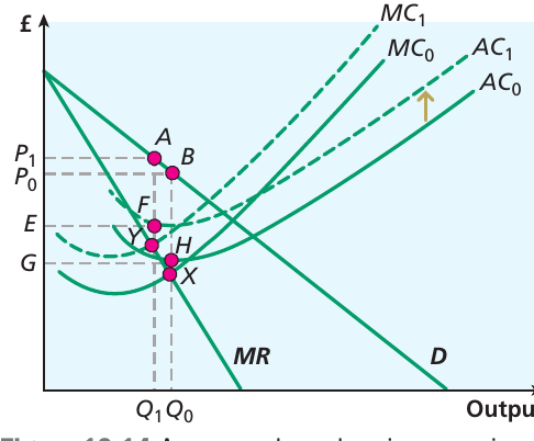
The original position has the firm maximising profits where at point X, setting price and producing output . The profit is given by the area .
When costs increase, the MC curve shifts up to , and the AC curve shifts up to . The firm now maximises profits where at point Y, setting a higher price and producing lower output . The profit area has shrunk to . Consumers must pay a higher price and can buy less of the good. The firm faces lower profits.
Important note: If the increase in average costs reflects an increase in fixed costs rather than variable costs, the profit-maximising output level would not change (since marginal costs haven't changed). However, profits would still be lower due to the higher fixed costs, with the firm simply charging the same price .
How monopolies arise
Monopolies can develop in a market for several different reasons.
Legal monopolies
In some instances, governments create monopolies through legal authority. For example, for 150 years the UK Post Office held a licence giving it a monopoly on delivering letters. This service was eventually opened to limited competition in the 2000s, though companies wishing to deliver packages weighing less than 350 grams and charging less than £1 could only do so by applying for a licence.
The patent system offers another form of legal protection. Patents are designed to provide an incentive for firms to innovate by developing new techniques and products. By prohibiting other firms from copying the product for a period of time (typically 20 years), the patent system gives firms a temporary monopoly. This allows them to earn supernormal profits as a reward for their innovation, encouraging further research and development.
Natural monopoly
A natural monopoly arises when the technology and cost structure of an industry creates substantial economies of scale throughout the relevant range of output. In such cases, there may only be room for one firm to operate efficiently in the market.
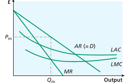
The diagram shows a natural monopoly situation. The key feature is that the long-run average cost (LAC) curve continues to decline throughout the range of market demand. The long-run marginal cost (LMC) curve lies below the LAC curve throughout this range.
This occurs when fixed costs of production are very high but marginal costs are low. For example, building a high-speed rail link like HS2 requires enormous expenditure on fixed costs (new track, upgraded stations, new rolling stock). However, once operational, the marginal cost of carrying an additional passenger is very low.
Any new entrant into such a market would necessarily operate at a lower scale than the existing firm, facing higher average costs. The existing firm can always price such competitors out of the market. These economies of scale therefore act as an effective barrier to entry, and the market becomes a natural monopoly.
A profit-maximising natural monopoly would produce at quantity (where ) and charge price .
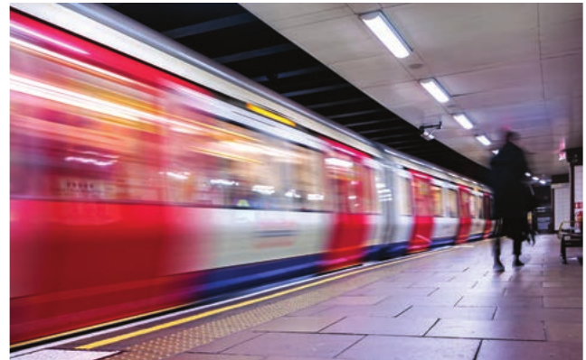
The London Underground is a classic example of a natural monopoly. The enormous fixed costs of building underground rail networks and tunnels, combined with relatively low marginal costs of running additional trains or carrying extra passengers, create the conditions for natural monopoly. It would not make economic sense to have parallel competing underground rail systems serving the same routes. Some cities (such as Kuala Lumpur) do have multiple rail systems, but they serve different routes rather than competing on the same routes.
Important note: The Channel Tunnel may appear to be an obvious natural monopoly, but it does face competition from ferry companies and airlines. The market is not a pure monopoly as there are substitute services available.
Competitive monopoly
Some firms have risen to become monopolies through their actions in the market rather than through legal protection or technological factors. This is sometimes called a competitive monopoly.
Firms may achieve monopoly status through effective marketing, establishing their product as a widely accepted standard, or through mergers and acquisitions. For example, by 2021, Google controlled more than 90% of the global search engine market, not through legal protection or natural monopoly conditions, but through establishing market dominance.
When firms merge (such as the Sainsbury's and Argos/Habitat merger), this can create synergies and reduce costs, but it may also lead to the combined firm gaining a monopoly position in certain markets.
Monopoly and efficiency
The characteristics of monopoly markets can be evaluated by examining different types of efficiency.
Productive efficiency
A firm achieves productive efficiency when it produces at the minimum point of its long-run average cost curve. This represents the lowest possible cost per unit of output.
Looking at the profit maximisation diagram, it is clear that productive efficiency is unlikely for a monopoly. The firm produces at quantity where , but this will only coincide with the minimum point of the LRAC curve by pure coincidence. If the marginal revenue curve happened to pass through exactly the minimum point of LRAC, productive efficiency would be achieved, but this would be a rare accident rather than a systematic outcome.
Furthermore, if a monopoly is protected by barriers to entry, the incentive to become and remain productively efficient may be weak. Without competitive pressure, complacency could lead to X-inefficiency - operating above minimum average cost due to organisational slack or inefficient management practices.
Allocative efficiency
Allocative efficiency occurs when price equals marginal cost (). At this point, the value consumers place on the last unit consumed (shown by the price they're willing to pay) equals the cost of producing that unit. Resources are optimally allocated from society's perspective.
A profit-maximising monopoly does not achieve allocative efficiency. The firm produces where , but because MR lies below the demand curve (AR), and AR represents price, we have . The monopolist charges a price above marginal cost.
In the profit maximisation diagram, the price is while marginal cost at that output level is , which is clearly lower. This means society values additional units more than they cost to produce, but the monopolist restricts output to keep prices high. This creates allocative inefficiency.
Dynamic efficiency
Dynamic efficiency refers to efficiency over time, particularly relating to innovation and technological progress. A firm achieves dynamic efficiency when it uses supernormal profits to invest in research and development, creating new products or reducing production costs in the future.
Monopolies may be able to achieve dynamic efficiency. Because they can earn supernormal profits, they have the financial resources available to invest in R&D. This may lead to cost reductions or new product development that benefits consumers in the long run.
However, dynamic efficiency is not guaranteed under monopoly. In the absence of competitive pressure, the firm may become complacent and allow X-inefficiency to develop rather than innovating. The monopolist's incentive to innovate depends on whether it faces potential competition from new technologies or substitute products.
This provides a contrast with perfect competition, where firms earn only normal profits and therefore lack the financial resources for substantial R&D investment, though they face strong competitive pressure to improve efficiency.
Comparing perfect competition and monopoly
We can identify the welfare effects of monopoly by comparing it with perfect competition operating under the same cost conditions. To simplify the analysis, let's assume no economies of scale, so we can use the same cost curves for both market structures.
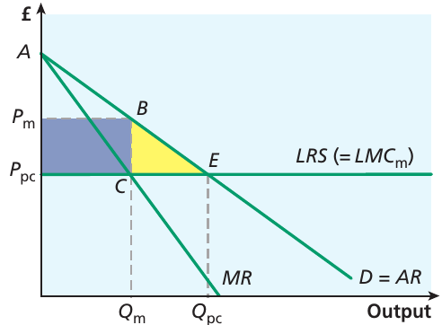
The diagram compares equilibrium outcomes under both market structures:
Under perfect competition: The market operates where the long-run supply curve () intersects the demand curve. The competitive equilibrium produces quantity at price . Consumer surplus is the entire area under the demand curve above the price - shown as the area .
Under monopoly: The profit-maximising monopolist produces where , resulting in quantity at price . Consumer surplus shrinks to the area . The purple/grey rectangular area represents a transfer from consumer surplus to producer surplus - this is profit earned by the monopolist that was previously consumer surplus.
Deadweight loss
The key welfare loss from monopolisation is shown by the yellow triangular area BCE. This is called deadweight loss - it represents a loss to society from the monopolisation of the industry. This welfare is lost entirely; it doesn't transfer to the monopolist but simply disappears from the economy.
The deadweight loss occurs because the monopolist restricts output below the socially optimal level. Units between and are valued by consumers (shown by the demand curve) more than they cost to produce (shown by the LRS curve), but the monopolist does not supply them because doing so would reduce profits.
Key insight: The monopolist produces less output than a perfectly competitive industry and charges a higher price, creating both a redistribution of welfare (from consumers to the firm) and a deadweight loss to society.
Summary of the comparison
When a profit-maximising monopoly operates under the same cost conditions as a perfectly competitive industry, it will:
- Produce less output ()
- Charge a higher price ()
- Create deadweight loss (area BCE)
- Transfer consumer surplus to producer surplus (area )
- Reduce overall economic welfare
Price discrimination
Are there any conditions in which a monopoly firm would produce the level of output consistent with allocative efficiency? The answer lies in understanding price discrimination.
Perfect (first-degree) price discrimination
Consider a market operated by a monopolist who faces constant marginal cost (). Under normal monopoly behaviour with a single price, the market outcome would be at price and quantity under perfect competition, but at price and quantity under monopoly.
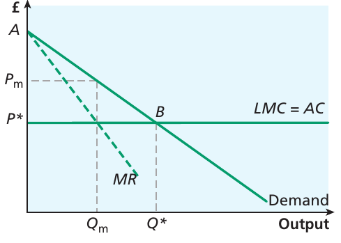
But suppose the monopolist could charge a different price to each individual consumer - charging each consumer exactly their maximum willingness to pay for the product. This is called perfect price discrimination or first-degree price discrimination.
In this scenario, the demand curve effectively becomes the marginal revenue curve, as it represents what the monopolist will receive for each unit sold (since each unit is sold at a different price). The firm would then maximise profits where MR (now equal to AR) intersects LMC - at point B in the diagram, producing quantity .
The outcome produces the allocatively efficient quantity! However, consumer surplus has been completely eliminated. The area that was consumer surplus () under perfect competition is no longer consumer surplus but becomes producer surplus - the monopolist has captured the entire original consumer surplus as its own profits.
From society's overall perspective, total welfare is the same as under perfect competition (though distributed very differently). However, this represents a massive redistribution from consumers to the monopolist. The monopolist has essentially hijacked all consumer benefits.
Reality check: Perfect price discrimination is quite rare in the real world, though it might exist in certain markets like art, fashion or designer jewellery where prices are individually negotiated between buyer and seller.
Third-degree price discrimination
More commonly observed is third-degree price discrimination, where a firm charges different prices to different groups of consumers rather than to each individual consumer separately.
Students, disabled people and older people in England may get discounted bus fares. Younger and older people may get cheaper access to sporting events or theatres. Railway passengers pay different prices for peak and off-peak travel. In all these cases, different consumer groups pay different prices for essentially the same product.
Key terms:
-
Third-degree price discrimination: A situation in which a firm is able to charge groups of consumers a different price for the same product
-
Arbitrage: A process by which prices in two market segments are equalised by the purchase and resale of products by market participants
Conditions for price discrimination
For a firm to successfully practise price discrimination, three conditions must be met:
-
Market power - The firm must have some degree of market power (the ability to set prices above marginal cost). Price discrimination is impossible in perfectly competitive markets where all sellers are price takers.
-
Information - The firm must have information about consumers and their willingness to pay. There must be identifiable differences between consumers or groups of consumers, particularly differences in their price elasticities of demand (different sensitivities to price).
-
Prevention of resale - Consumers must have limited ability to resell the product. If consumers could easily resell, those who qualified for the low price could buy up the product and resell it to consumers in other market segments, engaging in arbitrage. This would eliminate the price differences and undermine the discrimination strategy.
Memory aid: Remember MIP - Market power, Information, Prevention of resale.
How third-degree price discrimination works
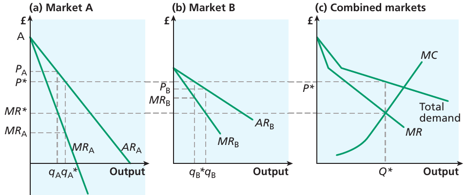
The diagram shows how a monopolist practices third-degree price discrimination across two markets (Market A and Market B):
If the firm had to charge the same price to all consumers, it would set marginal revenue equal to marginal cost in the combined market, producing output to be sold at price . The firm would sell units in Market A and units in Market B at this single price.
However, examining the two separate markets reveals an opportunity. In Market A, marginal revenue () is much lower than in Market B (). This difference in marginal revenue opens up a profit-increasing opportunity for the firm.
By taking sales away from Market A and selling more in Market B, the firm gains more extra revenue in B than it loses in A, increasing total profit. The optimal position occurs where marginal revenue is equalised across the two markets.
In the discriminating equilibrium, the firm sells units in Market A at the higher price , and units in Market B at the lower price . Notice that in both situations, the amounts sold in the two submarkets sum to - total output hasn't changed from the single-price scenario.
Key insight: The market with less elastic demand (Market A) faces the higher price, while the market with more elastic demand (Market B) faces the lower price.
Benefits for the firm
By undertaking price discrimination, the firm can increase its profits. The discriminating monopolist shown in the three-panel diagram separates two distinct groups of consumers with differing demand curves and different price elasticities. This allows the firm to extract more revenue from consumers with lower price elasticity (less sensitive to price changes) while still making sales to consumers with higher price elasticity (more sensitive to price changes).
In essence, price discrimination allows the monopolist to capture more consumer surplus and convert it into producer surplus (profit).
Benefits for consumers
Consumers in Market B (the low-price market) benefit from this practice, as they can now consume more of the good than they would at the single higher price. Indeed, without price discrimination, the price might be so high that these consumers would not be able to consume the good at all.
Furthermore, if the monopolist uses its higher profits for research and development, consumers may benefit from new and improved products or from cross-subsidisation of other services provided by the firm.
The Competition and Markets Authority (CMA) investigated the energy market and found wide price variation for electricity and gas, even though these are homogeneous products. Many customers could have saved money by switching suppliers, tariffs or payment methods. Average potential savings were equivalent to more than 20% of customers' bills. In 2018, the government accepted and began implementing remedies suggested by the CMA to address this issue.
Overall evaluation
Study tip: Be ready with the three conditions necessary for price discrimination: market power, information about different consumers and their elasticities of demand, and limited ability for consumers to resell the product.
Price discrimination creates both benefits and costs:
Benefits:
- Some consumers gain access to products that would otherwise be beyond their price range
- May lead to greater dynamic efficiency if profits fund R&D
- Can enable cross-subsidisation of other services
Costs:
- Reduces consumer surplus significantly
- Involves redistribution from consumers to producers
- May seem unfair that different groups pay different prices for the same product
Evaluation of monopoly
A profit-maximising monopoly firm produces less output at a higher price than would occur under perfect competition. Since the monopolist sets price above marginal cost, allocative efficiency is not achieved.
However, several considerations may moderate this negative assessment:
Potential benefits of monopoly:
-
Economies of scale: A monopoly may be able to exploit economies of scale that would not be available to smaller firms. By producing at lower cost, a firm with a monopoly in the home market may be better positioned to compete with firms in a global market environment.
-
Dynamic efficiency: The supernormal profits earned by a monopoly provide financial resources that can be used for research and development activity. This may lead to dynamic efficiency - innovation and technological progress over time. Under perfect competition, firms lack these resources for substantial R&D investment.
-
Natural monopoly efficiency: In industries with substantial fixed costs but low marginal costs, having multiple competing firms would be wasteful. A natural monopoly may produce at lower cost than would be possible under competition.
-
Price discrimination benefits: If a monopoly firm practises price discrimination, some consumers may gain access to products that would otherwise be beyond their financial reach. The discriminating monopolist may also produce closer to the allocatively efficient quantity.
Potential costs of monopoly:
-
Allocative inefficiency: Price exceeds marginal cost (), meaning society values additional units more than they cost to produce, but the monopolist restricts output to maintain high prices.
-
Lack of productive efficiency: The monopolist is unlikely to produce at minimum average cost and may not have strong incentives to minimise costs.
-
X-inefficiency: Without competitive pressure, the monopolist may become complacent, allowing organisational slack and inefficient management practices to develop.
-
Deadweight loss: The restriction of output below the competitive level creates a welfare loss to society that benefits no one.
-
Distributional effects: Monopoly power transfers consumer surplus to producer surplus. While this doesn't reduce total welfare (it's a transfer, not a loss), it may raise equity concerns about the distribution of economic benefits.
-
Reduced consumer choice: With only one supplier, consumers have no alternatives if they dislike the monopolist's product quality, customer service, or other characteristics.
Real-world complexity:
The practical assessment of any particular monopoly requires examining the specific circumstances of that market. The Competition and Markets Authority (CMA), the UK regulatory body responsible for monitoring monopoly markets, is empowered to investigate mergers if they result in the combined firm having more than 25% of a market. The CMA can examine whether the monopoly harms consumer welfare and recommend remedies if necessary.
Remember!
Key Points to Remember:
- A monopoly is a market with a single seller, protected by barriers to entry and facing no close substitutes for its product
- The monopolist is a price maker, facing the market demand curve directly and producing where to maximise profits
- Marginal revenue lies below average revenue for a monopolist; for a linear demand curve, MR has exactly twice the slope of AR
- Monopolists always produce in the elastic portion of the demand curve where marginal revenue is positive
- Barriers to entry allow monopolists to earn supernormal profits that persist in the long run
- A monopoly generally fails to achieve productive efficiency (minimum average cost) or allocative efficiency ()
- Compared to perfect competition, monopoly produces less output at a higher price, creating deadweight loss to society
- Natural monopolies arise from substantial economies of scale where only one firm can operate efficiently
- Price discrimination allows monopolists to charge different prices to different consumers, requiring market power, information about consumers, and prevention of resale
- Third-degree price discrimination charges different prices to different market segments, typically charging higher prices to groups with more inelastic demand
- While monopolies create allocative inefficiency and deadweight loss, they may achieve dynamic efficiency through innovation funded by supernormal profits