The multiplier and the accelerator (OCR A-Level Economics): Revision Notes
1.5 The multiplier and the accelerator
DEFINITIONS:
-
Multiplier effect: when a change in expenditure causes a greater final change in real GDP. To calculate it is the following equation:
-
Marginal Propensity to Withdraw (MPW): the proportion of the change in income that leaks out of the circular flow of income. To calculate:
-
Marginal Propensity to Import (MPM): the proportion of additional income that is allocated to import expenditure. To calculate:
-
Marginal Rate of Taxation (MRT): the proportion of additional income that is taxed. To calculate:
-
Average Propensity to Withdraw (APW): measures the ratio of withdrawals to total income. To calculate:
-
Average Propensity to Save (APS): the proportion of total income that is saved. To calculate:
-
Average Rate of Taxation (ART): the proportion of total income that is taxed. To calculate:
-
Average Propensity to Import (APM): the proportion of total income spent on imports. To calculate:
Explain
The concept of the multiplier became important in the 1930s when Keynes suggested it as a tool to maintain high levels of employment. To stimulate further rounds of spending, he suggested to inject new demand for goods and services into the circular flow of income. As a result, this has an even bigger impact on output and employment.
Factors affecting the multiplier:
- the multiplier effect would be smaller with large leakages in the circular flow of income
- the multiplier will be large provided that the MPW is low
- Below summarises the conditions under which the multiplier will be effective: | Component | Explanation | |---|---| | MPS | when MPS is low. the multiplier is large, as less income is allocated to saving | | MRT | when MRT is low, the multiplier is large as less income is taxed | | MPM | when MPM is low, the multiplier is large, as less income is allocated to import expenditure |
Explain with the aid of a diagram
1.5.2 The National Income Multiplier and Accelerator
National Income Multiplier:
Definition: The national income multiplier (often simply called the "multiplier") measures the ratio of the change in national income to the initial change in autonomous spending that caused it. It shows how an initial increase in spending leads to a larger overall increase in national income.
Formula: where MPC is the marginal propensity to consume.
Diagram:
Explanation: When there is an initial increase in autonomous spending (e.g., investment, government spending, or exports), this spending becomes someone else's income. A portion of this income will be spent on consumption (depending on the MPC), creating further income and consumption in successive rounds. The total impact on national income is a multiple of the initial change in spending.
The accelerator effect:
Definition: The accelerator effect refers to the relationship between the level of investment and the rate of change of national income. It posits that an increase in national income can induce firms to increase investment, particularly when they expect that the increase in demand will be sustained.
Explanation: The accelerator effect suggests that if national income is rising, firms expect future demand to increase, which encourages them to invest more to expand their productive capacity. Conversely, if national income is falling, firms reduce investment. The accelerator thus can amplify economic fluctuations, reinforcing the multiplier effect.
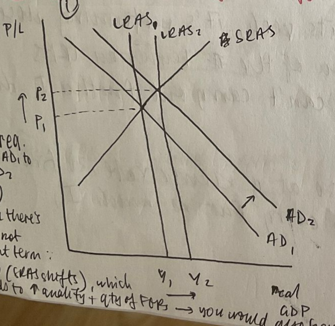
Keynesian economists believe the interaction of the multiplier and accelerator effect gives rise to the cyclical response to initial shocks. The key factor here is the level of investment. A change in national income and output enacts the accelerator effect, meaning investment increases. This increases AD and enacts the multiplier, causing further increases in output.
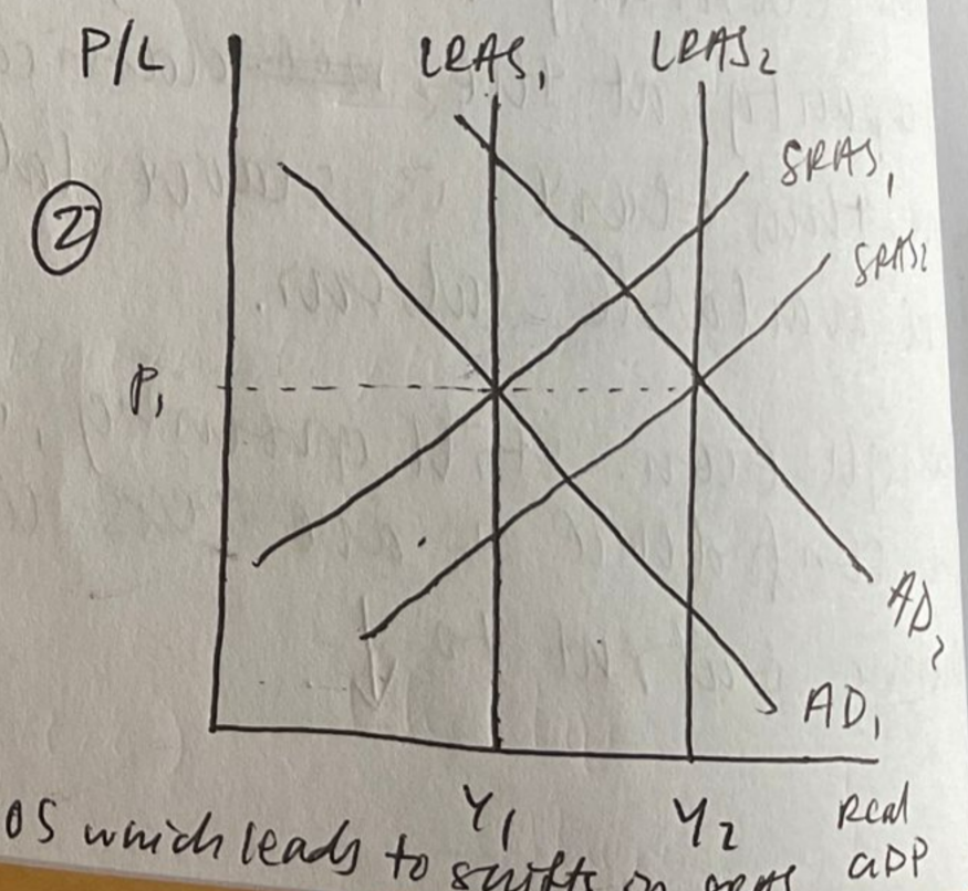
When there is an increase in economic growth as a result of an increase in AD, there is an incentive to increase investment, which in increases the productive capacity. Thus there is a fall in the cost to produce goods, shifting SRAS1 down to SRAS2
Combined Multiplier-Accelerator Interaction:
The interaction between the multiplier and the accelerator can lead to significant economic fluctuations. An initial autonomous increase in spending leads to a multiplied increase in national income, which then triggers further investment through the accelerator effect, causing a further increase in income, and so on.
A simplified flowchart can be used to show the relationship:
Step 1: Initial Increase in Autonomous Spending (ΔA) -> Multiplier Effect -> Increase in National Income (ΔY)
Step 2: Increase in National Income (ΔY) -> Accelerator Effect -> Increase in Investment (I)
Step 3: Increase in Investment (I) -> Further Increase in National Income (ΔY)
By understanding the multiplier and accelerator effects, economists can better predict the potential impacts of fiscal policies and other economic changes on the overall economy.
1.5.3 Explanation of the National Income Multiplier and Accelerator:
National Income Multiplier: The national income multiplier effect refers to the process by which an initial change in spending (such as investment, government expenditure, or exports) leads to a more than proportionate change in national income (GDP). This is because the initial spending creates income for others, who in turn spend part of this income, creating further income and spending, and so on.
Accelerator Effect: The accelerator effect explains how an increase in national income can lead to a proportionally larger increase in investment. Firms invest more when they expect higher future demand. Therefore, an increase in GDP (and aggregate demand) can stimulate more investment, which further boosts aggregate demand.
Aggregate Demand and Economic Cycle Diagram:
To illustrate the combined impact of the multiplier and accelerator on aggregate demand (AD) and the economic cycle, we use the following diagram:
Economic Cycle:
-
Expansion: The combined effects of the multiplier and accelerator can lead to a rapid increase in aggregate demand, causing an expansion phase in the economic cycle.
-
Peak: Eventually, the economy may reach a peak where resources are fully employed, and further increases in AD lead to inflation rather than real GDP growth.
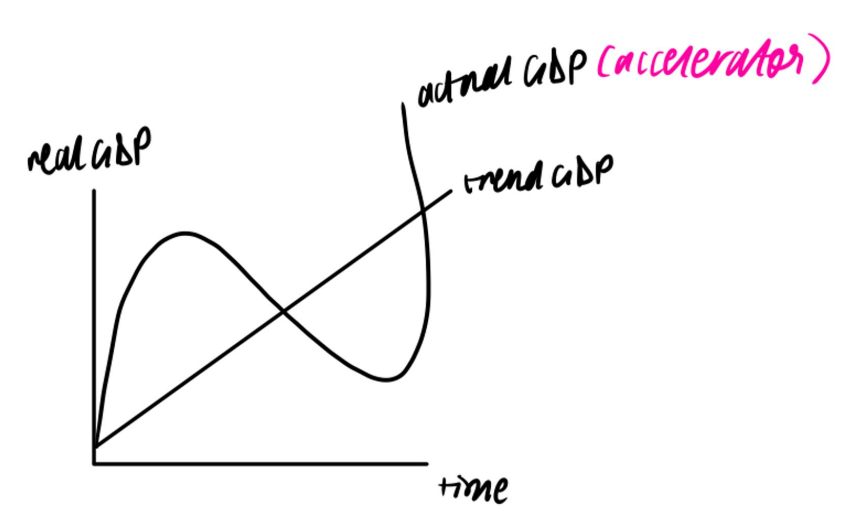
-
Contraction: If investment falls or consumption decreases, the reverse effects can lead to a contraction phase. The accelerator effect can amplify the downturn as lower GDP reduces investment.
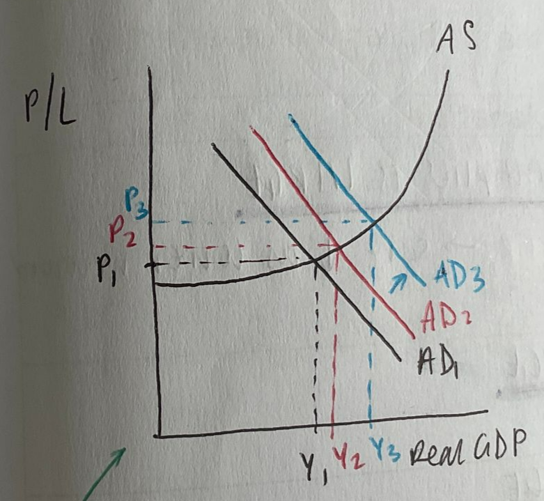
Impact on Aggregate Demand and Economic Cycle:
- Initial Increase in Investment (or other spending):
- Suppose there is an initial increase in investment (I1 to I2) due to business optimism or government policy.
- This shifts the AD curve from AD1 to AD2.
- Multiplier Effect:
- The initial increase in investment increases income and consumption, leading to a further increase in AD.
- The size of this effect depends on the multiplier. If the MPC is high, the multiplier effect is larger, leading to a more significant shift in AD.
- Accelerator Effect:
- The increase in national income (GDP) encourages firms to invest more, anticipating higher future demand.
- This additional investment further shifts AD to the right, potentially from AD2 to AD3 (not shown in the diagram for simplicity).
Summary:
The multiplier and accelerator effects together can significantly influence aggregate demand and the economic cycle. An initial increase in spending can lead to a multiplied increase in national income due to the multiplier effect, while the accelerator effect can further boost investment, amplifying the impact on aggregate demand. These dynamics contribute to the cyclical nature of the economy, with periods of expansion and contraction.
1.5.4 Output Gaps, Aggregate Demand and Aggregate Supply Model, and a Production Possibility Curve (PPC)
Output Gap: An output gap is the difference between the actual output of an economy and its potential output. It can be either positive or negative:
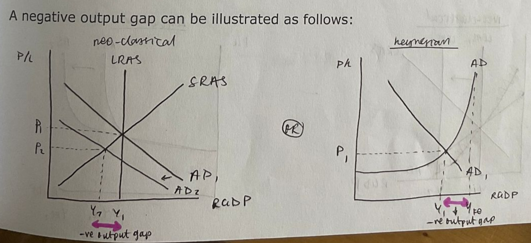
- Negative Output Gap (Recessionary Gap): Actual output is below potential output, indicating underutilised resources and unemployment.
- Positive Output Gap (Inflationary Gap): Actual output exceeds potential output, suggesting an overheated economy with potential inflationary pressures.
Aggregate Demand and Aggregate Supply (AD-AS) Model:
- Equilibrium: Where AD intersects AS.
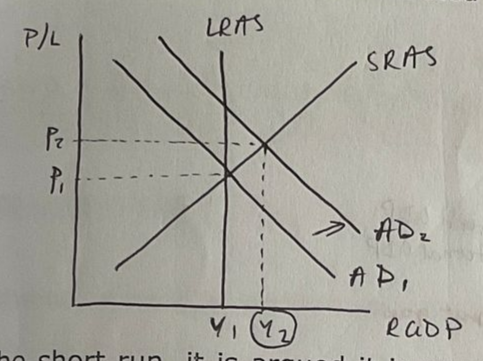
- Positive Output Gap: When actual output (Y2) is greater than potential output (Y*).
The AD-AS model illustrates the relationship between the aggregate demand and aggregate supply in an economy and the resulting equilibrium output and price level.
- Negative Output Gap: When actual output (Y1) is less than potential output (Y*).
Production Possibility Curve (PPC):
The PPC illustrates the maximum possible output combinations of two goods or services an economy can achieve when all resources are fully and efficiently utilised.
Key Points:
- Points on the Curve: Efficient use of resources.
- Points inside the Curve: Inefficient use of resources (negative output gap).
- Points outside the Curve: Currently unattainable with existing resources (positive output gap).
Diagram:
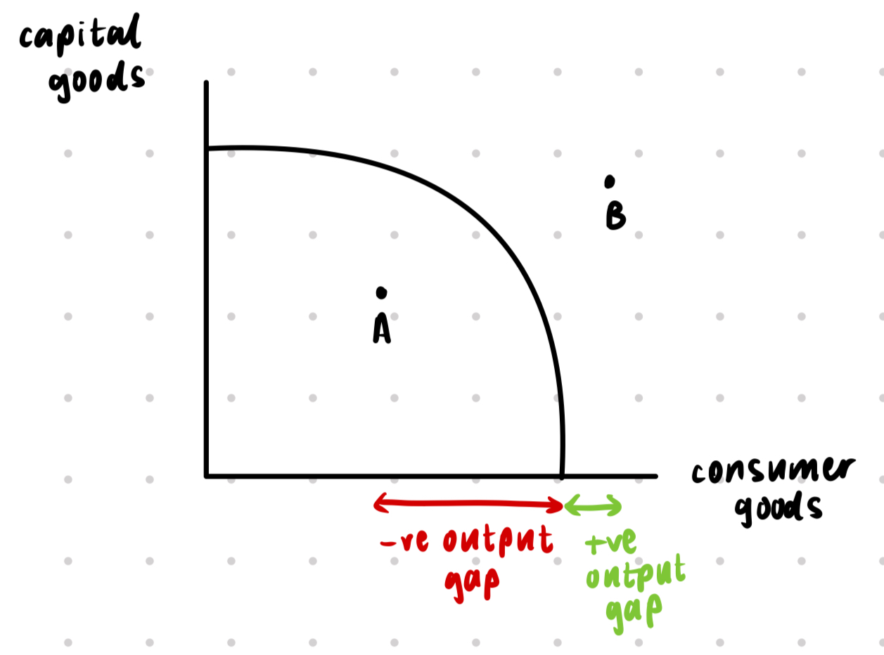
- On the PPC: Economy is producing efficiently.
- Inside the PPC: Economy is not utilising all resources efficiently (negative output gap).
- Outside the PPC: Economy is overextending beyond its capacity (positive output gap).
Explanation with Diagram Integration:
- Negative Output Gap:
- AD-AS Model: When AD is lower, actual output is below potential output (Y1 < Y*), indicating underutilization of resources.
- PPC: Economy operates inside the curve.
- Positive Output Gap:
- AD-AS Model: When AD is higher, actual output exceeds potential output (Y2 > Y*), indicating overutilization of resources and potential inflationary pressures.
- PPC: Economy operates beyond the curve, though this is unsustainable in the long term.
Explain & Calculate
1.5.5 Average and marginal propensities to consume, save and withdraw
Average and Marginal Propensities
In economics, the concepts of average and marginal propensities to consume, save, and withdraw are essential for understanding consumer behaviour and economic activity.
1. Average Propensity to Consume (APC)
Definition: The Average Propensity to Consume (APC) is the proportion of total income that households spend on consumption.
Formula:
Where:
- C is consumption.
- Y is total income.
2. Average Propensity to Save (APS)
Definition: The Average Propensity to Save (APS) is the proportion of total income that households save.
Formula:
Where:
- S represents savings.
- Y represents total income.
3. Marginal Propensity to Consume (MPC)
Definition: The Marginal Propensity to Consume (MPC) is the proportion of any additional income that households spend on consumption.
Formula:
Where:
- = change in consumption
- = change in income
4. Marginal Propensity to Save (MPS)
Definition: The Marginal Propensity to Save (MPS) is the proportion of any additional income that households save.
Formula:
5. Marginal Propensity to Withdraw (MPW)
Definition: The Marginal Propensity to Withdraw (MPW) is the proportion of any additional income that is withdrawn from the circular flow of income. This includes savings, taxes, and imports.
Formula:
where:
- is the Marginal Propensity to Tax
- is the Marginal Propensity to Import.
Example Calculations
Suppose a household's total income increases from £50,000 to £60,000. As a result, their consumption increases from £40,000 to £46,000, and their savings increase from £10,000 to £14,000.
Calculate APC:
Calculate APS:
Calculate MPC:
Calculate MPS:
Interpretation
- APC of 0.767 means that, on average, 76.7% of the household's income is spent on consumption.
- APS of 0.233 means that, on average, 23.3% of the household's income is saved.
- MPC of 0.6 means that for every additional £1 of income, the household spends 60p on consumption.
- MPS of 0.4 means that for every additional £1 of income, the household saves 40p.
1.5.6 National Income Multiplier
Formula:
The size of the national income multiplier can be calculated using the marginal propensity to consume (MPC) or the marginal propensity to save (MPS).
or
where:
- MPC (Marginal Propensity to Consume): The proportion of additional income that households spend on consumption.
- MPS (Marginal Propensity to Save): The proportion of additional income that households save (MPS = 1 - MPC).
Calculation Steps:
- Determine the MPC: This is usually given or can be calculated based on consumption and income data.
- Calculate the Multiplier: Use the formula k = 1 / (1 - MPC).
Example Calculation:
Suppose the MPC is 0.8.
- Calculate the Multiplier:
This calculation shows how to find the multiplier using an MPC of 0.8. The result is a multiplier of 5.
These represent the multiplier () in economics, which shows how an initial change in spending leads to a larger change in the overall economy. The multiplier can be calculated using either the Marginal Propensity to Consume (MPC) or the Marginal Propensity to Save (MPS).
Interpretation:
A multiplier of 5 means that an initial increase in autonomous spending (e.g., government spending or investment) will ultimately increase the national income by five times the initial amount.
Practical Example:
If the government increases its spending by £100 million and the MPC is 0.8:
Initial Increase in Spending: £100 million.
Total Increase in National Income:
This calculation shows how to find the total increase in national income by multiplying the multiplier by the increase in government spending . In this case, the total increase in national income is £500 million. So, a £100 million increase in government spending will result in a £500 million increase in national income.