Estimating Probabilities from Experiments Revision Notes for Leaving Cert Mathematics

Estimating Probabilities from Experiments

Introduction to experimental probability

When we calculated probabilities earlier, we assumed all outcomes were equally likely to happen. However, in real-life situations, events are not always equally likely and we need another method to estimate the probability of an event occurring.

In such cases, we carry out an experiment or survey to estimate the probability of an event happening. This is called experimental probability.

infoNote

Experimental probability is particularly useful when dealing with real-world situations where we cannot assume equal likelihood of outcomes, such as weather patterns, consumer preferences, or manufacturing defects.

Understanding relative frequency

When we conduct experiments to estimate probability, we use a concept called relative frequency.

Relative frequency is the number of times an event occurs divided by the total number of trials. It gives us an estimate of the probability that the event will happen.

The relative frequency formula

chatImportant

Essential Formula

$\text{Relative frequency} = \frac{\text{Number of successful trials}}{\text{Total number of trials}}$

This value provides an estimate of the probability that an event will occur by carrying out a survey or experiment.

The law of large numbers

An important principle in probability is that as the number of trials or experiments increases, the value of the relative frequency gets closer to the true or theoretical probability.

infoNote

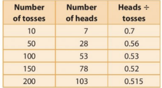
This table shows how a coin toss experiment demonstrates this principle. Notice how the ratio of heads approaches 0.5 (the theoretical probability) as more tosses are made. This convergence illustrates why larger sample sizes are always preferable in probability experiments.

Worked example 1: Car colour survey

Let's examine a practical example of experimental probability.

Derek collects data on the colours of cars passing the school gate. His results are shown below:

lightbulbExample

Worked Example: Analysing Car Colour Data

Table

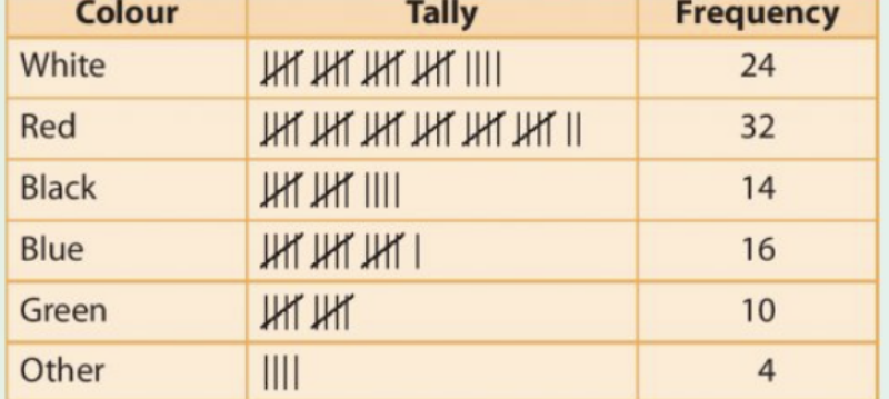
(i) Total cars surveyed = 24 + 32 + 14 + 16 + 10 + 4 = 100 cars

(ii) Relative frequency of blue cars = $\frac{16}{100} = \frac{4}{25} = 0.16$

(iii) Relative frequency of red cars = $\frac{32}{100} = 0.32$

(iv) Probability that next car will be green = relative frequency of green cars = $\frac{10}{100} = \frac{1}{10} = 0.1$

(v) The estimate for the probability of green cars can be made more reliable by increasing the sample size. Observing 500 cars would give a more accurate estimate of the true probability.

Expected frequency

Sometimes we need to predict how many times an event will occur in a given number of trials. This is called expected frequency.

chatImportant

Expected Frequency Formula

Expected frequency = probability × number of trials

Example calculation

If the probability of getting a blue disc from a bag is $\frac{2}{5}$ , then in 50 draws, the expected number of blue discs is:

$\text{Expected frequency} = \frac{2}{5} \times 50 = 20$

Worked example 2: Biassed dice

lightbulbExample

Worked Example: Biassed Dice Probability

A biassed dice has the following probability distribution:

Number	1	2	3	4	5	6
Probability	0.1	0.1	0.2	a	0.2	0.3

Part (i): Finding the missing probability

Since the dice must land on one of the numbers 1 to 6, the sum of all probabilities equals 1:

$0.1 + 0.1 + 0.2 + a + 0.2 + 0.3 = 1$ $0.9 + a = 1$ $a = 1 - 0.9 = 0.1$

Part (ii): Expected number of sixes

If the dice is thrown 300 times: Expected number of sixes = P(6) × number of trials = 0.3 × 300 = 90

Worked example 3: Spinner experiment results

Four friends test a spinner with different numbers of spins:

lightbulbExample

Worked Example: Comparing Reliability of Results

Name	Number of spins	Results
		0	1	2
Alan	30	12	12	6
Keith	100	31	49	20
Bill	300	99	133	68
Ann	150	45	73	32

Which results are most reliable?

Bill's results are most likely to give the best estimate because he conducted the most trials (300). According to the law of large numbers, more trials produce more reliable probability estimates.

infoNote

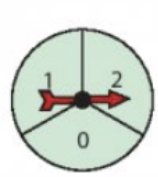
The spinner diagram shows a simple probability tool commonly used in experiments. When testing such devices, remember that the reliability of your probability estimates depends heavily on your sample size.

Key tips for exam success

chatImportant

Critical Exam Points

Always check that probabilities in a distribution add up to 1
Larger sample sizes give more reliable estimates
Relative frequency gives an estimate, not the exact probability
Show all working when calculating expected frequencies
Compare experimental and theoretical probabilities to identify bias

Common exam scenarios

Understanding these typical question types will help you prepare effectively:

Identifying bias: Compare experimental results to expected theoretical outcomes
Missing probabilities: Use the fact that probabilities sum to 1
Expected frequency: Multiply probability by number of trials
Sample size: Larger samples give more reliable estimates

infoNote

Practice identifying which type of question you're dealing with first. This will help you choose the correct approach and formula to apply.

bookmarkSummary

Key Points to Remember:

Relative frequency = Number of successful outcomes ÷ Total number of trials
Expected frequency = Probability × Number of trials
The sum of all probabilities in a complete distribution equals 1
Larger sample sizes produce more reliable probability estimates
Experimental probability approaches theoretical probability as trials increase

Estimating Probabilities from Experiments (Leaving Cert Mathematics): Revision Notes