Advanced Formatting (Grade 11 NSC Matric Computer Application Technology): Revision Notes
Advanced Formatting
Advanced formatting in spreadsheets is like giving your data superpowers! It helps you make your spreadsheets not just functional, but visually appealing and easy to understand. When you master these techniques, you'll be able to create professional-looking documents that automatically highlight important information and save you loads of time.
Conditional formatting
Conditional formatting is one of the most powerful features in spreadsheet applications like Excel. Think of it as creating "smart" formatting that automatically changes the appearance of cells based on their content. Instead of manually highlighting cells one by one, you set up rules that do the work for you.
What is conditional formatting?
Understanding Conditional Formatting
Conditional formatting automatically applies formatting to cells when they meet specific conditions. For example, you might want all test scores above 90% to appear in green, or all overdue dates to show in red. The spreadsheet checks each cell's value and applies the formatting if it matches your criteria.
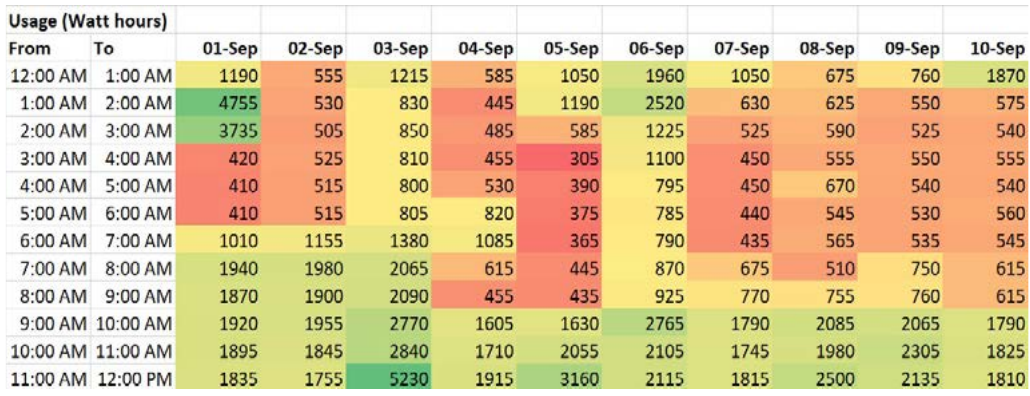
This energy monitoring table shows how conditional formatting can transform raw data into an easy-to-read visual format using colour coding.
Types of conditional formatting rules
There are five main types of conditional formatting rules, each designed for different purposes:
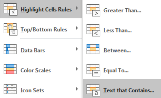
Highlight cells rules are the most commonly used type. These allow you to highlight data based on specific conditions such as:
- Values greater than or less than a certain number
- Values between two numbers
- Text that contains specific words
- Duplicate values
- Cells that are empty or contain errors
Top/Bottom rules help you identify extreme values in your data. You can highlight:
- The top 10 or bottom 10 values
- The top 10% or bottom 10% of values
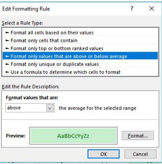
- Values that are above or below average
This is particularly useful for teachers tracking student performance or businesses identifying their best and worst performing products.
Data bars add coloured bars inside cells that act like mini bar charts. The length of each bar represents the value in that cell compared to other values in the selection. Larger values get longer bars, making it easy to spot trends at a glance.
Colour scales use gradients to show how values relate to each other. Cells with higher values might appear in darker colours, while lower values appear lighter. This creates a heat map effect that's perfect for showing patterns in large datasets.
Icon sets add small symbols to cells based on their values. You might use arrows pointing up, down, or sideways to show trends, or use traffic light colours (red, yellow, green) to indicate performance levels.
Applying conditional formatting
The process of applying conditional formatting follows a consistent pattern regardless of which type you choose.
Let's look at a practical example using highlight cells rules:
Worked Example: Highlighting High Grades
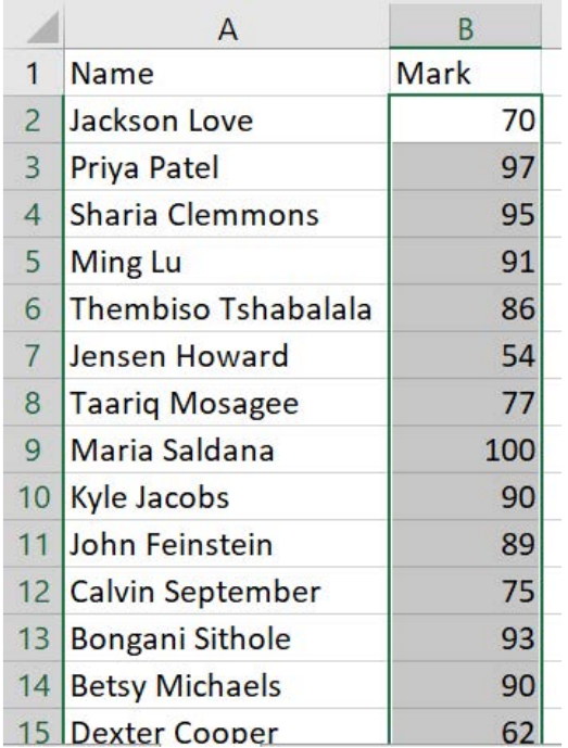
Suppose you want to highlight all student marks above 90 in a grades spreadsheet. Here's how you'd do it:
Step 1: Select your data range - Choose the cells containing the marks you want to format
Step 2: Access conditional formatting - Go to the Home tab and click on Conditional Formatting
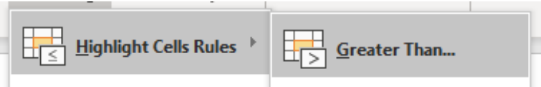
Step 3: Choose your rule type - Select "Highlight Cells Rules" then "Greater Than"
Step 4: Set your condition - Enter 90 in the dialogue box
Step 5: Choose your formatting - Pick a colour scheme (like light red fill with dark red text)
Step 6: Apply the rule - Click OK to see the formatting applied automatically
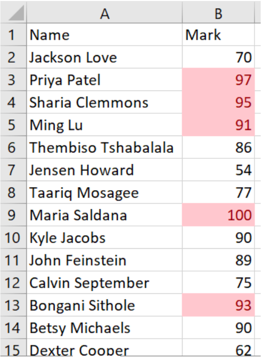
The result is a spreadsheet where all marks above 90 are immediately visible with special formatting.
Text-based conditional formatting
You can also format cells based on text content. This is useful when working with categories or labels.

Worked Example: Highlighting Team Sports
If you have a sports team roster and want to highlight all soccer players:
Step 1: Select the sport column
Step 2: Choose "Highlight Cells Rules" then "Text that Contains"
Step 3: Type "Soccer" in the dialogue box
Step 4: Choose your formatting style
Step 5: Apply the rule
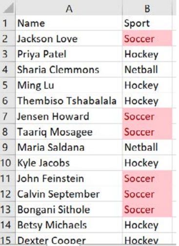
Now all cells containing "Soccer" will be highlighted, making it easy to identify soccer players in your roster.
Managing conditional formatting rules
Once you've applied conditional formatting, you might need to modify or remove rules later. The "Manage Rules" feature lets you:
- Edit existing rules to change conditions or formatting
- Delete rules you no longer need
- Change the order in which rules are applied
- See all rules applied to your worksheet
Managing Complex Formatting
This is particularly useful when working with complex spreadsheets that have multiple formatting rules. Always review your rules to ensure they don't conflict with each other.
AutoFill options
AutoFill is like having a smart assistant that can predict what data you want to enter next. It's designed to save you time by automatically filling in patterns of data.
Understanding AutoFill
When you need to enter a series of numbers, dates, or even custom lists, AutoFill can do the heavy lifting for you. Instead of typing each entry manually, you provide a pattern and let AutoFill complete the sequence.
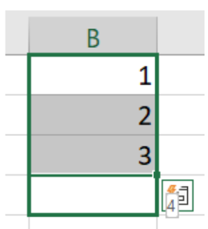
The fill handle is the small square that appears in the bottom-right corner of a selected cell. When you hover over it, your cursor changes to a thin black cross.
How to use AutoFill
Worked Example: Using AutoFill
The basic AutoFill process involves these steps:
Step 1: Enter your starting pattern - Type the first few values in your series (like 1, 2 for numbers or Monday, Tuesday for days)
Step 2: Select the cells - Highlight the cells containing your pattern
Step 3: Drag the fill handle - Click and drag the small square in the corner of your selection
Step 4: Choose your option - If needed, select from the AutoFill options that appear
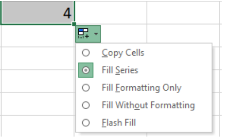
AutoFill options explained
When you use AutoFill, you'll often see a dropdown menu with different options for how to complete your series:
Copy Cells simply repeats the same values over and over. If you start with "Apple", it will fill "Apple, Apple, Apple..."
Fill Series creates a logical sequence. Starting with 1, 2 creates 3, 4, 5... or starting with January, February creates March, April, May...
Fill Formatting Only copies just the visual formatting (colours, fonts, borders) without copying the actual values.
Fill Without Formatting copies the values but leaves the formatting as it was in the destination cells.
Flash Fill is particularly clever - it looks at patterns in your data and tries to complete them automatically. For example, if you type "Smith, John" then "Jones, Mary", it might recognise you're formatting names as "Last, First".
Fill Days, Fill Weekdays, Fill Months, Fill Years are specialised options for working with dates and times.
Absolute cell referencing
Understanding cell referencing is crucial for creating formulas that work correctly when copied to different locations in your spreadsheet.
Relative vs absolute references
By default, spreadsheet formulas use relative references. This means that when you copy a formula from one cell to another, the cell references adjust automatically based on the new location.
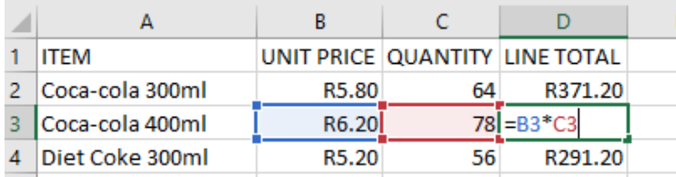
Understanding Relative References
For example, if cell D3 contains the formula =B3*C3, and you copy this to cell D4, it automatically becomes =B4*C4.
When to use absolute references
Sometimes you don't want references to change when you copy a formula. This is where absolute references come in handy. You create an absolute reference by adding dollar signs ($) before the column letter, row number, or both.
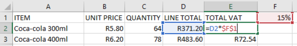
Consider a VAT calculation where the VAT rate is stored in cell F1 (15%). You want to calculate VAT for multiple products, but the rate should always refer to F1, not move to F2, F3, etc.
Types of absolute references
There are three ways to use the dollar sign in references:
Worked Example: Types of Absolute References
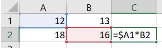
Fully absolute ($A$1) - Both the column (A) and row (1) are fixed. This reference will never change when copied.
Column absolute ($A1) - The column (A) is fixed, but the row (1) can change. Useful when you always want to reference column A but allow the row to adjust.
Row absolute (A$1) - The row (1) is fixed, but the column (A) can change. Useful when you always want to reference row 1 but allow the column to adjust.
Practical example of absolute referencing
Let's say you're calculating VAT for multiple products:
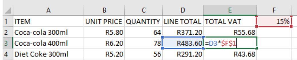
Worked Example: VAT Calculation with Absolute References
In cell E2, you might enter the formula =D2*$F$1. This multiplies the line total (D2) by the VAT rate in F1. The dollar signs ensure that when you copy this formula down to other rows, it will always reference cell F1 for the VAT rate, while the D2 part will adjust to D3, D4, etc.
When copied to row 3, the formula becomes =D3*$F$1 - perfect for calculating VAT for each product while always using the same rate.
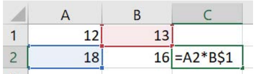
Mixed references in action
Mixed references are particularly powerful in tables where you need to fix either the row or column but not both.
Understanding Mixed References
For example, $A1*B$2 creates a reference where:
- Column A is always used (due to $A)
- Row 2 is always used (due to $2)
- But the other parts can adjust when copied
This is useful for creating multiplication tables or when working with data that has fixed headers or constants along one axis.
Key Points to Remember:
- Conditional formatting automatically applies visual formatting based on cell values, making data patterns easy to spot
- Use the five main rule types - Highlight Cells, Top/Bottom Rules, Data Bars, Colour Scales, and Icon Sets - for different data visualisation needs
- AutoFill saves time by automatically completing patterns in data series, dates, and custom lists
- The dollar sign ($) creates absolute references that don't change when formulas are copied to new locations
- Mixed references give you precise control over which parts of a reference stay fixed when copying formulas