Multiple Transformations Revision Notes for HSC SSCE Mathematics Advanced

Multiple Transformations

What are multiple transformations?

When we work with functions, we often need to apply more than one transformation to a parent function. Multiple transformations combine different types of changes—translations (shifts), reflections (flips), and dilations (stretches or compressions)—to create a new, more complex function. Understanding how to apply these transformations in the correct order is essential for finding the equation of the transformed function and sketching its graph accurately.

infoNote

Multiple transformations allow us to create complex functions from simple parent functions by applying a sequence of geometric changes. Each transformation modifies the function in a specific way, and combining them creates powerful tools for modeling real-world situations.

The importance of order

When applying multiple transformations, the order in which you apply them makes a significant difference to the final result. Always follow the order specified in the question.

chatImportant

Key rule: If no specific order is given, apply dilations and reflections first, then apply translations.

This default order ensures consistency and helps avoid errors when working with transformed functions.

Worked example 1: Transforming a reciprocal function

Let's transform the reciprocal function $f(x) = \frac{1}{x}$ by applying the following sequence:

Reflect over the y-axis
Dilate vertically by a factor of 2
Translate left by 3 units
Translate up by 1 unit

Finding the equation of the transformed function

We need to apply each transformation step by step, following the given order.

lightbulbExample

Worked Example: Applying Multiple Transformations to a Reciprocal Function

Step 1: Write the parent function

$f(x) = \frac{1}{x}$

Step 2: Reflect over the y-axis (replace $x$ with $-x$ )

$f(-x) = \frac{1}{-x}$

Step 3: Dilate vertically by 2 (multiply the function by 2)

$2f(-x) = 2\left(\frac{1}{-x}\right)$

Step 4: Translate left by 3 (replace $x$ with $x + 3$ )

$2f(-(x + 3)) = \frac{2}{-(x + 3)} = \frac{-2}{x + 3}$

Step 5: Translate up by 1 (add 1 to the entire function)

$2f(-(x + 3)) + 1 = \frac{-2}{x + 3} + 1$

Step 6: Simplify the expression

$= -\frac{2}{x + 3} + 1$

The transformed function is:

$g(x) = -\frac{2}{x + 3} + 1$

Finding the vertical asymptote

A vertical asymptote occurs where the denominator of a rational function equals zero, as the function becomes undefined at these points.

For $g(x) = -\frac{2}{x + 3} + 1$ , we need to find where $x + 3 = 0$

x + 3 = 0 x = -3

The vertical asymptote is at $x = -3$ .

Finding the horizontal asymptote

For reciprocal functions, the horizontal asymptote is determined by the constant term that was added or subtracted during vertical translation.

The parent function $f(x) = \frac{1}{x}$ has a horizontal asymptote at $y = 0$ .

Since we translated the function up by 1 unit, the horizontal asymptote moves from $y = 0$ to:

$y = 0 + 1 = 1$

The horizontal asymptote is at $y = 1$ .

Determining the domain and range

Domain: The domain includes all real numbers except where the denominator equals zero (the vertical asymptote).

Domain: $x \neq -3$ , or in interval notation: $(-\infty, -3) \cup (-3, \infty)$

Range: The range includes all real numbers except the horizontal asymptote value.

Range: $y \neq 1$ , or in interval notation: $(-\infty, 1) \cup (1, \infty)$

Sketching the transformed graph

To sketch the graph accurately, we need to find the intercepts and plot key points.

Finding the y-intercept (substitute $x = 0$ ):

g(x) = -\frac{2}{x + 3} + 1 g(0) = -\frac{2}{0 + 3} + 1 = -\frac{2}{3} + 1 = \frac{1}{3}

The y-intercept is at $\left(0, \frac{1}{3}\right)$ .

Finding the x-intercept (set $g(x) = 0$ ):

g(x) = -\frac{2}{x + 3} + 1 0 = -\frac{2}{x + 3} + 1 -1 = -\frac{2}{x + 3} x + 3 = 2 x = -1

The x-intercept is at $(-1, 0)$ .

Finding an additional point: To help sketch the branch that doesn't intersect the x-axis or y-axis, we can substitute $x = -4$ :

g(-4) = -\frac{2}{-4 + 3} + 1 = -\frac{2}{-1} + 1 = 2 + 1 = 3

Another point on the graph is $(-4, 3)$ .

infoNote

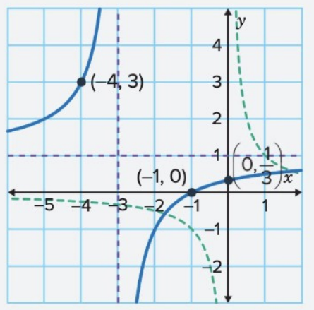
The complete graph shows:

A hyperbola with two branches
Vertical asymptote: $x = -3$ (shown as a vertical dashed line)
Horizontal asymptote: $y = 1$ (shown as a horizontal dashed line)
Key points: $(-4, 3)$ , $(-1, 0)$ , and $\left(0, \frac{1}{3}\right)$
One branch curves from the upper left towards both asymptotes
The other branch curves from the lower right towards both asymptotes

The asymptotes have shifted from their original positions at $x = 0$ and $y = 0$ to $x = -3$ and $y = 1$ , confirming that our transformations were applied correctly.

Worked example 2: Transforming a quadratic function

Let's transform the quadratic function $f(x) = x^2$ by applying the following sequence:

Dilate horizontally by a factor of $\frac{1}{2}$
Reflect over the x-axis
Translate right by 2 units
Translate down by 1 unit

Finding the equation of the transformed function

We apply each transformation in the given order.

lightbulbExample

Worked Example: Applying Multiple Transformations to a Quadratic Function

Step 1: Write the parent function

$f(x) = x^2$

Step 2: Dilate horizontally by $\frac{1}{2}$ (replace $x$ with $\frac{x}{\frac{1}{2}} = 2x$ )

Note: A horizontal dilation by factor $\frac{1}{2}$ means we replace $x$ with $\frac{x}{\frac{1}{2}}$ , which makes the graph wider.

f\left(\frac{x}{\frac{1}{2}}\right) = f(2x) = (2x)^2 = 4x^2 f(2x) = 4x^2

Step 3: Reflect over the x-axis (multiply by -1)

$-f(2x) = -4x^2$

Step 4: Translate right by 2 (replace $x$ with $x - 2$ )

$-f(2(x - 2)) = -4(x - 2)^2$

Step 5: Translate down by 1 (subtract 1 from the function)

$-f(2(x - 2)) - 1 = -4(x - 2)^2 - 1$

The transformed function is:

$g(x) = -4(x - 2)^2 - 1$

Finding the vertex

The transformed function is now in vertex form: $y = a(x - h)^2 + k$

In this form, the vertex is located at the point $(h, k)$ .

For $g(x) = -4(x - 2)^2 - 1$ :

$h = 2$ (remember the sign is opposite in the formula)
$k = -1$

The vertex is at $(2, -1)$ .

chatImportant

In vertex form $y = a(x - h)^2 + k$ , the signs can be tricky! The vertex is at $(h, k)$ , but notice that in the equation, we have $(x - h)$ , not $(x + h)$ . So if you see $(x - 2)^2$ , then $h = 2$ (positive), not -2.

Determining the range

The range of a parabola depends on two factors:

The sign of $a$ (which determines whether the parabola opens upward or downward)
The value of $k$ (the y-coordinate of the vertex)

For $g(x) = -4(x - 2)^2 - 1$ :

$a = -4$ , which is negative
Since $a < 0$ , the parabola is concave down (opens downward)
The vertex represents the maximum point

Therefore, the range is: $(-\infty, -1)$ or $y \leq -1$

Sketching the transformed graph

To sketch an accurate graph, we need to find intercepts and additional points.

Finding the y-intercept (substitute $x = 0$ ):

g(x) = -4(x - 2)^2 - 1 g(0) = -4(0 - 2)^2 - 1 = -4 \times 4 - 1 = -16 - 1 = -17

The y-intercept is at $(0, -17)$ .

Finding the x-intercept (set $g(x) = 0$ ):

g(x) = -4(x - 2)^2 - 1 0 = -4(x - 2)^2 - 1 4(x - 2)^2 = -1 (x - 2)^2 = -\frac{1}{4}

Since $(x - 2)^2 \geq 0$ for all real values of $x$ , this equation has no solution.

There are no x-intercepts.

infoNote

The fact that there are no x-intercepts makes sense because the parabola opens downward with its maximum point (vertex) at $(2, -1)$ , which is below the x-axis. The entire parabola lies below the x-axis, so it never crosses it.

Finding an additional point: Since there's only one intercept, we need another point to help sketch the parabola accurately. Let's try $x = 3$ :

g(x) = -4(x - 2)^2 - 1 g(3) = -4(3 - 2)^2 - 1 = -4(1)^2 - 1 = -4 - 1 = -5

Another point on the graph is $(3, -5)$ .

infoNote

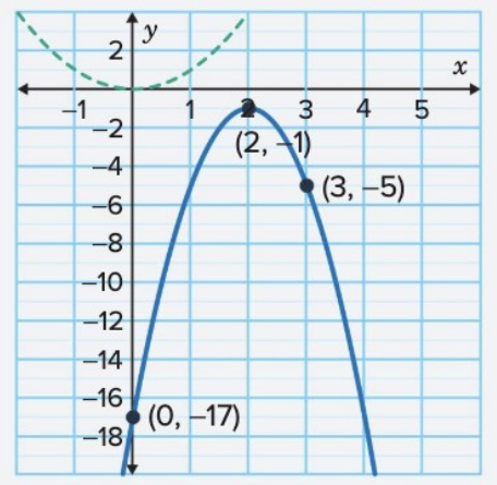
The complete graph shows:

An inverted (concave down) parabola
Vertex at $(2, -1)$ (the maximum point)
y-intercept at $(0, -17)$
No x-intercepts
Additional point at $(3, -5)$
The parabola is wider than the parent function $y = x^2$ due to the horizontal dilation

The vertex has shifted from the origin $(0, 0)$ to $(2, -1)$ , and the graph is now inverted and wider, confirming all our transformations have been applied correctly.

Remember!

bookmarkSummary

Key Points to Remember:

Order matters: Always apply transformations in the order specified. If no order is given, apply dilations and reflections before translations.
Build step by step: Apply one transformation at a time and write out each step clearly to avoid errors.
Check key features: After finding the transformed equation, verify your work by checking asymptotes (for rational functions), vertices (for quadratics), intercepts, domain, and range.
Sketch with landmarks: When drawing the transformed graph, always plot asymptotes (for rational functions), vertices (for quadratics), intercepts, and at least one additional point to ensure accuracy.
Connect to the parent function: Understanding how the transformations affect the parent function's key features helps you predict what the transformed graph should look like.

Multiple Transformations (HSC SSCE Mathematics Advanced): Revision Notes