Exponential Graphs (HSC SSCE Mathematics Advanced): Revision Notes
Exponential Graphs
Introduction
An exponential function is a special type of function where the variable appears in the exponent (the power). These functions have unique properties and create distinctive curved graphs that you'll learn to recognise and sketch. Understanding exponential functions is essential because they model many real-world situations, from population growth to radioactive decay.
Exponential functions appear everywhere in the real world: bacteria populations doubling every hour, radioactive substances decaying over time, compound interest growing in savings accounts, and the spread of viral content on social media. Understanding their behaviour helps you model and predict these phenomena.
Key terminology
Before exploring exponential graphs, you need to understand some important terms:
Exponential function: A function written in the form , where is the variable and the base is a positive number.
Exponential growth: This occurs when a quantity increases at a rate that is proportional to its current value. The larger the quantity becomes, the faster it grows.
Exponential decay: This occurs when a quantity decreases at a rate that is proportional to its current value. As the quantity gets smaller, it decreases more slowly.
Asymptote: A line that a curve approaches but never actually touches, no matter how far the graph extends. For exponential functions, this is typically a horizontal line.
Domain: The complete set of input values (-values) that are allowed in a function. For exponential functions, this includes all real numbers.
Range: The complete set of output values (-values) that a function can produce.
Key features of exponential functions
The general form of an exponential function is , where , , and .
The base must be positive and cannot equal 1. If , the function becomes , which is just a horizontal line, not an exponential function. The constant cannot be zero, otherwise the function would be for all values of .
This function has several important characteristics:
Y-intercept: The graph crosses the -axis at the point . This is because when , we have .
Horizontal asymptote: The line (the -axis) acts as a horizontal asymptote. As moves towards negative or positive infinity, the graph approaches this line but never touches it.
Domain: All real numbers. You can substitute any real number for .
Range: All values where (when ). The function never produces negative values or zero.
Exponential growth
When the base is greater than 1 (that is, ), the function shows exponential growth. As increases, the -values increase at an accelerating rate.
Let's examine the function as an example. Here's a table showing how the -values change:
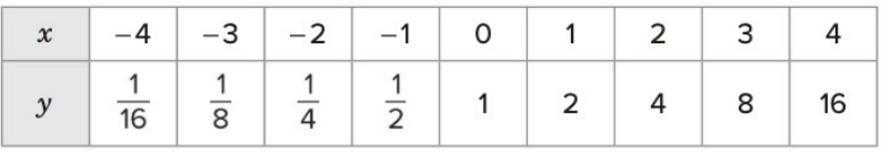
Notice that as increases by 1, the -values double each time. This doubling pattern is characteristic of exponential growth. When the base is 3, values triple; when the base is 4, they quadruple, and so on.
When we plot these points on a graph, we get a distinctive J-shaped curve:
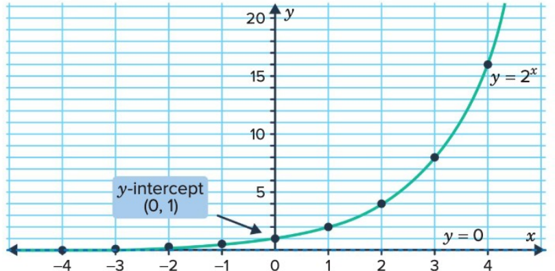
The graph shows several key features:
- The curve passes through the point , which is the -intercept
- As increases (moving right), the curve rises steeply
- As decreases (moving left), the curve approaches the -axis but never touches it
- The horizontal asymptote is at
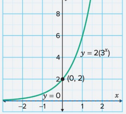
Worked example 1: Identifying features of
Worked Example: Identifying features of
Let's work through identifying the key features of the function .
Finding the horizontal asymptote:
As , we have
Therefore
The horizontal asymptote is
Finding the y-intercept:
Substitute :
The -intercept is at the point
Finding the domain:
The domain is all real numbers, since we can substitute any real number for .
Finding the range:
Since for all values of , and
We have
The range is
Sketching the graph:
To sketch this function, follow these steps:
-
Plot the -intercept at
-
Draw the horizontal asymptote as a dashed line
-
Calculate additional points:
At :
At :
-
Draw a smooth curve through the points, showing exponential growth to the right and approaching the asymptote to the left
Exponential decay
When the base is between 0 and 1 (that is, ), the function shows exponential decay. As increases, the -values decrease and approach zero.
The function is equivalent to . This form represents exponential decay and creates a graph that is a reflection of the growth function across the -axis.
The negative exponent in "flips" the base to its reciprocal. For example, is the same as . This transformation converts a growth function into a decay function.
Worked example 2: Exploring
Worked Example: Exploring
Let's complete a table of values for from to .
Calculating y-values:
For :
For :
For :
For :
The completed table shows:
Analysing the behaviour:
Since :
As , (the function increases without bound)
As , (the function approaches zero from above)
The horizontal asymptote is
The domain is all real numbers
The range is
Worked example 3: Comparing growth and decay with
Worked Example: Comparing growth and decay with
Let's examine the function and compare it to .
Creating a table of values:
Calculate for values from to :
Describing the behaviour:
As increases, the -values halve each time. This represents exponential decay, with values decreasing at a rate that slows down as they approach zero.
Sketching and comparing:
When we plot both and on the same graph:
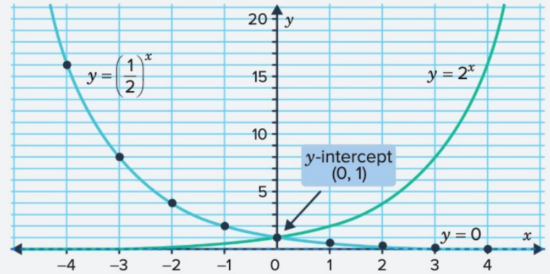
Key observations:
- Both graphs pass through (the -intercept)
- The graph of increases to the right (growth)
- The graph of decreases to the right (decay)
- Both have the horizontal asymptote
- The graphs are reflections of each other across the -axis
Behaviour of exponential functions
The behaviour of exponential functions depends on the base and the scaling factor .
For where :
When (exponential growth):
- As , (the function increases without limit)
- As , (the function approaches zero from above)
When (exponential decay):
- As , (the function approaches zero from above)
- As , (the function increases without limit)
For :
This form is equivalent to , which reverses the behaviour due to the factor . If in the original function, then , converting growth into decay.
Exam tips
Essential Tips for Exam Success:
- Always check whether (growth) or (decay) before sketching
- The -intercept is easy to find: just substitute
- Remember that the asymptote for basic exponential functions is always
- When comparing exponential functions, larger bases grow more rapidly
- Make sure your curve is smooth and continuous, not angular or broken
- The domain is always all real numbers unless otherwise restricted
Key Points to Remember:
- Exponential functions have the form where and
- If , the function shows exponential growth; if , it shows exponential decay
- All exponential functions of this form have a -intercept at and a horizontal asymptote at
- The domain is all real numbers, and the range is (when )
- As increases, growth functions rise rapidly whilst decay functions approach zero