Quadratic and Cubic Functions (HSC SSCE Mathematics Advanced): Revision Notes

Worked Example 1: Graphing $f(x) = 2x^3$

Let's graph $f(x) = 2x^3$ by finding key points and understanding the function's behavior.

Strategy:

We'll substitute several $x$-values into the function to find corresponding $y$-values, then plot these points. Since $k = 2 > 0$, we know the graph will increase from bottom-left to top-right through these points.

Solution:

Choose $x$-values of $-1$, $0$, and $1$ to find key points:

When $x = -1$:

$f(-1) = 2(-1)^3$

$f(-1) = 2(-1)$

$f(-1) = -2$

This gives us the point $(-1, -2)$.

When $x = 0$:

$f(0) = 2(0)^3$

$f(0) = 0$

This gives us the point $(0, 0)$.

When $x = 1$:

$f(1) = 2(1)^3$

$f(1) = 2$

This gives us the point $(1, 2)$.

Since $k = 2 > 0$, the graph increases from bottom-left to top-right, passing through these points.

The domain is $\mathbb{R}$ and the range is $\mathbb{R}$, as the function is continuous and unbounded.

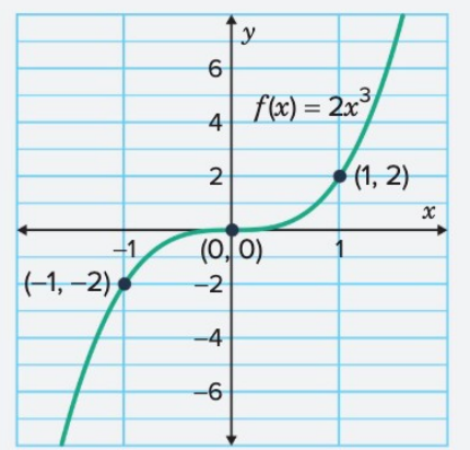
The graph shows the characteristic S-shaped curve of a cubic function, increasing through the key points $(-1, -2)$, $(0, 0)$, and $(1, 2)$.

Worked Example 2: Analyzing $f(x) = (x + 2)(x - 1)(x - 3)$

Let's work through finding the intercepts, domain, range, and graph for this factored cubic function.

Part a: Find the x- and y-intercepts

Strategy for x-intercepts:

Set $f(x) = 0$ and solve for $x$ using the factored form.

Solution for x-intercepts:

$(x + 2)(x - 1)(x - 3) = 0$

Using the null factor law, set each factor equal to zero:

$x + 2 = 0$, or $x - 1 = 0$, or $x - 3 = 0$

$x = -2$, or $x = 1$, or $x = 3$

The x-intercepts are at $(-2, 0)$, $(1, 0)$, and $(3, 0)$.

Strategy for y-intercept:

Substitute $x = 0$ into the function to find where the graph crosses the y-axis.

Solution for y-intercept:

$f(0) = (0 + 2)(0 - 1)(0 - 3)$

$f(0) = (2)(-1)(-3)$

$f(0) = 6$

The y-intercept is at $(0, 6)$.

Part b: Determine the domain and range

Since the function is not restricted by any practical context, the domain is $\mathbb{R}$ and the range is $\mathbb{R}$.

Part c: Graph the function

Strategy:

Plot the intercepts found in part (a), and use the domain and range from part (b) to understand the graph's extent.

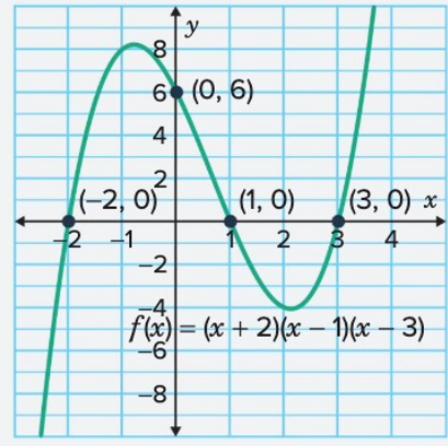
The graph shows a cubic curve with x-intercepts at $(-2, 0)$, $(1, 0)$, and $(3, 0)$, and y-intercept at $(0, 6)$. The function increases overall since the implied coefficient is positive.

Worked Example 3: Volume of a Box

A box is made from a $10$ cm by $6$ cm piece of cardboard by cutting squares of side $x$ cm from each corner. The volume is given by:

$V(x) = 4x(3 - x)(5 - x) \text{ cm}^3$

Part a: Determine the practical domain for which the volume is positive

Strategy:

Find where $V(x) = 0$ by solving for the roots. Divide the number line into intervals using these roots. Test a point in each interval to determine where $V(x) > 0$. Finally, apply the physical constraints of the problem to find the practical domain.

Solution:

First, find the roots by setting $V(x) = 0$:

$4x(3 - x)(5 - x) = 0$

Using the null factor law:

$x = 0$, or $x = 3$, or $x = 5$

These roots divide the number line into intervals: $(-\infty, 0)$, $(0, 3)$, $(3, 5)$, and $(5, \infty)$.

Now test a point in each interval to determine where $V(x) > 0$:

The volume is positive over the intervals $(0, 3)$ and $(5, \infty)$.

However, we must consider the physical constraints. The shorter side of the cardboard is $6$ cm. If we cut squares of side $x$ cm from each corner, we remove $2x$ cm from this dimension (one square from each end). For the box to have positive width:

$6 - 2x > 0$

$6 > 2x$

$3 > x$

Therefore, $x$ must be less than $3$ cm. Additionally, $x$ must be positive. Combining these constraints with our mathematical analysis, the practical domain is $(0, 3)$.

Part b: Find the x- and y-intercepts

Strategy:

For x-intercepts, set $V(x) = 0$ and check which roots fall within the practical domain. For the y-intercept, evaluate $V(0)$.

Solution for x-intercepts:

From part (a), we know the mathematical x-intercepts are at $x = 0$, $x = 3$, and $x = 5$.

Within the practical domain $(0, 3)$, there are no x-intercepts because the interval is open (doesn't include the endpoints). The values $x = 0$ and $x = 3$ are boundary points where $V(x) = 0$, but they're not included in the practical domain.

Solution for y-intercept:

$V(0) = 4(0)(3-0)(5-0)$

$V(0) = 0$

The y-intercept is at $(0, 0)$, which is an endpoint of the practical domain.

Part c: Graph the function

Strategy:

Calculate additional points within the practical domain $(0, 3)$, then plot these along with the boundary behavior.

Solution:

Calculate $V(1)$:

$V(1) = 4 \times 1 \times (3-1)(5-1)$

$V(1) = 4 \times 2 \times 4$

$V(1) = 32$

This gives the point $(1, 32)$.

Calculate $V(2)$:

$V(2) = 4 \times 2 \times (3-2)(5-2)$

$V(2) = 8 \times 1 \times 3$

$V(2) = 24$

This gives the point $(2, 24)$.

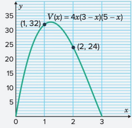
The graph shows the volume function for $0 < x < 3$, with points at $(1, 32)$ and $(2, 24)$. The volume approaches zero at the boundaries $x = 0$ and $x = 3$. Based on these points, the range is estimated as $(0, 32]$, indicating the maximum volume occurs somewhere between $x = 1$ and $x = 2$.