Continuous Distributions Revision Notes for HSC SSCE Mathematics Advanced

Continuous Distributions

Introduction to continuous distributions

In a continuous probability distribution, the random variable can take any value within an interval on the number line. Unlike discrete distributions where we can list all possible values, continuous distributions have infinitely many possible values.

Key features of continuous distributions:

The domain is typically a closed interval like $[0, 6]$
There are infinitely many possible values within the interval
The probability of any single specific value is exactly zero: $P(X = h) = 0$
Instead, we calculate probabilities over intervals: $P(2 \leq X \leq 5)$

chatImportant

This fundamental difference means we cannot use the tabular methods from discrete probability distributions. Instead, we need to use cumulative frequency and integration techniques.

The cumulative distribution function

The cumulative distribution function (CDF) tells us the probability that a random variable is less than or equal to a particular value.

Definition: For a continuous random variable $X$ with values from a closed interval $[a, b]$ , the cumulative distribution function is:

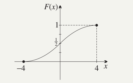
$F(x) = P(a \leq X \leq x), \text{ for all } x \text{ in } [a, b]$

infoNote

Properties of the CDF:

$F(x)$ is continuous
$F(x)$ is non-decreasing (never goes down)
$F(a) = 0$ (probability at the start is zero)
$F(b) = 1$ (probability at the end is one)
Can be used to calculate medians, quartiles, and percentiles

Example: the chook problem

lightbulbExample

Worked Example: The Chook Problem

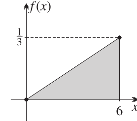
A chook wanders randomly in a circular enclosure of radius 6 metres. We want to find the probability distribution for its distance from the centre.

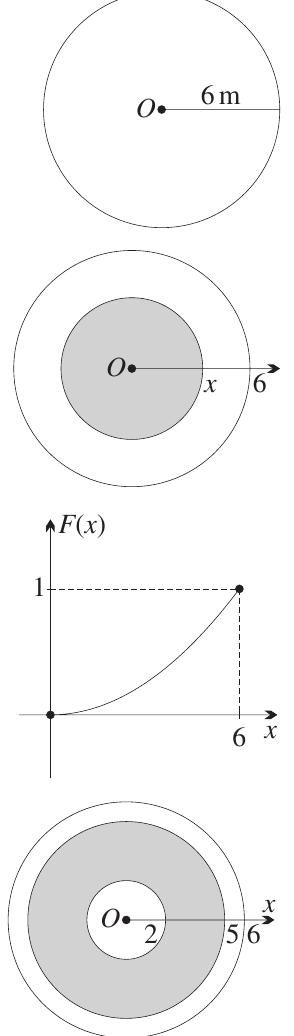
Let $F(x)$ be the probability that the chook is no more than $x$ metres from the centre:

$F(x) = \frac{\text{area of inner circle}}{\text{area of whole circle}} = \frac{\pi x^2}{\pi \times 6^2} = \frac{x^2}{36}, \text{ where } 0 \leq x \leq 6$

This function increases smoothly from $F(0) = 0$ to $F(6) = 1$ .

Using the CDF to find probabilities

We can find the probability of being in a range by subtracting CDF values:

$P(\text{chook is 2-5 metres from centre}) = F(5) - F(2) = \frac{25}{36} - \frac{4}{36} = \frac{21}{36}$

Finding quartiles and median

To find quartiles and median, we solve $F(x)$ for specific probability values:

lightbulbExample

Worked Example: Finding Quartiles and Median

First quartile ( $Q_1$ ): Set $F(x) = \frac{1}{4}$

$\frac{x^2}{36} = \frac{1}{4}$ $x^2 = 9$ $x = 3$

Median ( $Q_2$ ): Set $F(x) = \frac{1}{2}$

$\frac{x^2}{36} = \frac{1}{2}$ $x^2 = 18$ $x \approx 4.24$

Third quartile ( $Q_3$ ): Set $F(x) = \frac{3}{4}$

$\frac{x^2}{36} = \frac{3}{4}$ $x^2 = 27$ $x \approx 5.20$

The probability density function

The probability density function (PDF) is obtained by differentiating the CDF. It represents the "density" of probability at each point.

From CDF to PDF

Since addition becomes integration in continuous distributions, the CDF is the integral of the PDF. By the fundamental theorem of calculus, the PDF is the derivative of the CDF:

$f(x) = F'(x)$

lightbulbExample

Worked Example: Finding the PDF

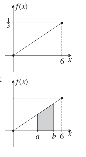
For our chook example:

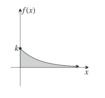
$f(x) = \frac{d}{dx}\left(\frac{x^2}{36}\right) = \frac{x}{18}, \text{ where } 0 \leq x \leq 6$

Interpreting the PDF

chatImportant

The PDF does not give the probability at a specific point (which is always zero). Instead, it allows us to calculate probabilities over intervals by integration.

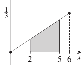
Key principle: The probability over an interval equals the area under the PDF curve:

$P(a \leq x \leq b) = \int_a^b f(x)\,dx$

Calculating probabilities using the PDF

lightbulbExample

Worked Example 1: Probability the chook is 2-5 metres from centre:

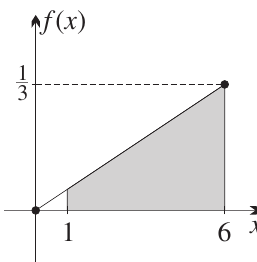
$P(2 \leq x \leq 5) = \int_2^5 \frac{x}{18}\,dx = \left[\frac{x^2}{36}\right]_2^5 = \frac{25-4}{36} = \frac{21}{36}$

lightbulbExample

Worked Example 2: Probability the chook is at least 1 metre from centre:

$P(x \geq 1) = \int_1^6 \frac{x}{18}\,dx = \left[\frac{x^2}{36}\right]_1^6 = \frac{36-1}{36} = \frac{35}{36}$

lightbulbExample

Worked Example 3: Total probability over entire domain:

$P(0 \leq X \leq 6) = \int_0^6 \frac{x}{18}\,dx = \left[\frac{x^2}{36}\right]_0^6 = \frac{36-0}{36} = 1$

Properties of probability density functions

A function $f(x)$ is a probability density function if it satisfies two conditions:

infoNote

Requirements for a Valid PDF:

1. Non-negative: $f(x) \geq 0$ for all $x$ in $[a, b]$

2. Total area equals one: $\int_a^b f(x)\,dx = 1$

These properties ensure that $f(x)$ represents valid probabilities.

Additional concepts

Mode: A global maximum of the PDF is called a mode. It represents the most "dense" region of probability.

chatImportant

Because $P(X = h) = 0$ for any specific value $h$ , it doesn't matter whether we use $\leq$ or $<$ in interval notation. The intervals $[2, 4]$ and $(2, 4)$ have the same probability.

The CDF as a signed area function

We can now formally define the relationship between PDF and CDF using integration.

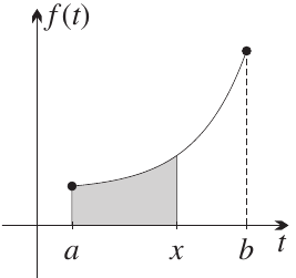
Given a PDF $f(x)$ on domain $[a, b]$ , the CDF is the signed area function:

$F(x) = \int_a^x f(t)\,dt, \text{ for } a \leq x \leq b$

Conversely, $f(x) = F'(x)$ (except possibly at isolated sharp corners).

infoNote

Remember: Be precise with terminology - "density" means at a point (PDF), and "distribution" means over a range (CDF).

Uniform continuous distributions

A uniform continuous distribution is one where the PDF is constant across the entire domain. This represents situations where all values in the interval are equally likely.

Properties of uniform distributions

For a uniform distribution on interval $[a, b]$ :

$f(x) = \frac{1}{b-a}$

The constant value ensures the total area under the curve equals 1.

Example: train waiting time

lightbulbExample

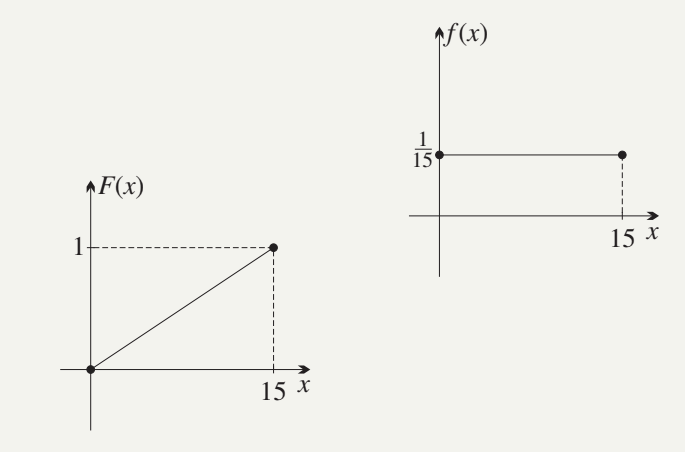
Worked Example: Train Waiting Time

Tran arrives at a station at a random time. Trains leave every 15 minutes. What is the probability distribution of his waiting time?

Solution:

The waiting time $x$ can be anything from 0 to 15 minutes. Since all waiting times are equally likely:

$f(x) = \frac{1}{15}, \text{ for } 0 \leq x \leq 15$

The CDF is found by integrating:

$F(x) = \int_0^x \frac{1}{15}\,dt = \left[\frac{t}{15}\right]_0^x = \frac{x}{15}$

Finding the median:

Set $F(x) = \frac{1}{2}$ :

$\frac{x}{15} = \frac{1}{2}$ $x = 7.5 \text{ minutes}$

Finding the 45th percentile:

Set $F(x) = \frac{45}{100} = \frac{9}{20}$ :

$\frac{x}{15} = \frac{9}{20}$ $x = 6.75 \text{ minutes}$

Probability of waiting 5-10 minutes:

Either integrate the PDF or use the CDF:

Method 1 (using PDF): $P(5 \leq X \leq 10) = \int_5^{10} \frac{1}{15}\,dt = \frac{10-5}{15} = \frac{1}{3}$

Method 2 (using CDF): $P(5 \leq X \leq 10) = F(10) - F(5) = \frac{10}{15} - \frac{5}{15} = \frac{1}{3}$

Piecewise-defined probability density functions

Some PDFs are defined differently on different parts of their domain. These require careful handling when integrating.

Example: a symmetric piecewise PDF

lightbulbExample

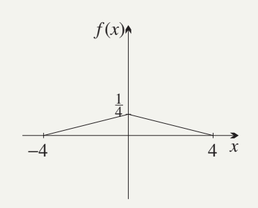
Worked Example: Symmetric Piecewise PDF

Consider the PDF:

$f(x) = \begin{cases} k(4+x), & \text{for } -4 \leq x \leq 0 \\ k(4-x), & \text{for } 0 \leq x \leq 4 \end{cases}$

Step 1: Find the constant $k$

The total area under the curve must equal 1. We integrate over both pieces:

$\int_{-4}^4 f(x)\,dx = \int_{-4}^0 k(4+x)\,dx + \int_0^4 k(4-x)\,dx$

$= k\left[4x + \frac{x^2}{2}\right]_{-4}^0 + k\left[4x - \frac{x^2}{2}\right]_0^4$

$= k(0 - (-16+8)) + k((16-8) - 0) = 16k$

Setting this equal to 1: $k = \frac{1}{16}$

Therefore:

$f(x) = \begin{cases} \frac{1}{16}(4+x), & \text{for } -4 \leq x \leq 0 \\ \frac{1}{16}(4-x), & \text{for } 0 \leq x \leq 4 \end{cases}$

Step 2: Calculate probabilities

To find $P(0 \leq X \leq 2)$ , we only need the right-hand branch:

$P(0 \leq X \leq 2) = \frac{1}{16}\int_0^2 (4-x)\,dx = \frac{1}{16}\left[4x - \frac{x^2}{2}\right]_0^2 = \frac{1}{16}(8-2) = \frac{3}{8}$

Step 3: Find median and mode

The median is 0 because the areas to the left and right of $x = 0$ are equal.

The mode is also $x = 0$ because this is where the PDF reaches its maximum value.

Step 4: Find the piecewise CDF

For $-4 \leq x \leq 0$ :

$F(x) = \frac{1}{16}\int_{-4}^x (4+t)\,dt = \frac{1}{32}[(4+t)^2]_{-4}^x = \frac{1}{32}(4+x)^2$

For $0 \leq x \leq 4$ , we note that $F(0) = \frac{1}{2}$ , then:

$F(x) = \frac{1}{2} + \frac{1}{16}\int_0^x (4-t)\,dt = \frac{1}{2} - \frac{1}{32}[(4-t)^2]_0^x = 1 - \frac{1}{32}(4-x)^2$

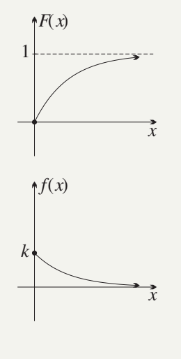
Distributions with unbounded domains

In many real-world situations, the PDF extends to infinity. This happens when there's a horizontal asymptote, meaning values can theoretically extend indefinitely (though with decreasing probability).

Example: radioactive decay

lightbulbExample

Worked Example: Radioactive Decay

The isotope iodine-131 has a half-life of 8 days. If we observe a single nucleus, the time $X$ (in days) before it decays follows an exponential distribution.

Using the half-life property:

$P(X > 8) = \frac{1}{2}, \quad P(X > 16) = \frac{1}{4}, \quad P(X > 24) = \frac{1}{8}$

This leads to the CDF:

$F(x) = 1 - e^{-kx}, \text{ where } k = \frac{\ln 2}{8} \approx 0.08664$

Finding the PDF:

Differentiate the CDF:

$f(x) = F'(x) = ke^{-kx}$

Domain: The domain is the unbounded interval $[0, \infty)$ because decay could theoretically occur at any time in the future.

Finding the median:

Set $F(x) = 0.5$ :

1 - e^{-kx} = \frac{1}{2} \\ e^{-kx} = \frac{1}{2} \\ -kx = \ln\frac{1}{2} = -\ln 2 \\ x = \frac{\ln 2}{k} = 8 \text{ days}

The median equals the half-life, as expected.

Calculating probabilities:

Probability of decay on first day: $P(X \leq 1) = F(1) = 1 - e^{-k} \approx 0.083$

Probability of decay after first day: $P(X > 1) = 1 - P(X \leq 1) = e^{-k} \approx 0.917$

Improper integrals (challenge)

When the domain extends to infinity, we use improper integrals. These involve taking limits as we approach infinity.

infoNote

Verifying the PDF integrates to 1:

For $f(x) = ke^{-kx}$ on $[0, \infty)$ :

$\int_0^\infty ke^{-kx}\,dx = \left[-e^{-kx}\right]_0^\infty$

At $x = 0$ : the value is $-1$

As $x \to \infty$ : the limit of $-e^{-kx}$ is $0$

Therefore: $\int_0^\infty ke^{-kx}\,dx = 0 - (-1) = 1$

lightbulbExample

Worked Example: Consider $f(x) = \frac{1}{x^2}$ on $[1, \infty)$

$\int_1^\infty \frac{1}{x^2}\,dx = \left[-\frac{1}{x}\right]_1^\infty$

At $x = 1$ : the value is $-1$

As $x \to \infty$ : the limit is $0$

Therefore: $\int_1^\infty \frac{1}{x^2}\,dx = 0 - (-1) = 1$

This shows $f(x) = \frac{1}{x^2}$ is a valid PDF on $[1, \infty)$ .

The CDF would be:

$F(x) = \int_1^x \frac{1}{t^2}\,dt = \left[-\frac{1}{t}\right]_1^x = 1 - \frac{1}{x}$

chatImportant

Counter-example with $f(x) = \frac{1}{x}$ :

$\int_1^\infty \frac{1}{x}\,dx = \left[\ln x\right]_1^\infty$

As $x \to \infty$ : $\ln x \to \infty$

This integral does not converge, so $f(x) = \frac{1}{x}$ cannot be a PDF on $[1, \infty)$ .

Key formulas summary

bookmarkSummary

Key Formulas to Remember:

Cumulative distribution function: $F(x) = P(X \leq x) = \int_a^x f(t)\,dt$

Probability density function: $f(x) = F'(x)$

Properties of PDF:

$f(x) \geq 0$ for all $x$
$\int_a^b f(x)\,dx = 1$

Probability over an interval: $P(h \leq X \leq k) = \int_h^k f(x)\,dx = F(k) - F(h)$

Uniform distribution on $[a, b]$ : $f(x) = \frac{1}{b-a}$

Remember!

bookmarkSummary

Key Points to Remember:

In continuous distributions, the probability of any single value is zero
The CDF starts at 0 and ends at 1, and is always non-decreasing
The PDF must be non-negative, and its total area must equal 1
Probability equals area under the PDF curve
"Density" refers to a point (PDF), "distribution" refers to a range (CDF)
Quartiles and median are found by setting $F(x)$ equal to $\frac{1}{4}$ , $\frac{1}{2}$ , and $\frac{3}{4}$ respectively

Continuous Distributions (HSC SSCE Mathematics Advanced): Revision Notes