Decay and Half-Life Revision Notes for HSC SSCE Physics

Decay and Half-Life

Introduction to radioactive decay

Radioactive decay is a naturally occurring process where unstable atomic nuclei spontaneously break down and emit radiation. What makes this process particularly interesting is its random nature. When you have a single radioactive nucleus, it's impossible to predict exactly when it will decay, or even whether it will decay during a specific time period.

infoNote

Think of it like tossing a coin. You cannot predict whether a single coin will land on heads or tails. Similarly, you cannot predict when an individual radioactive nucleus will decay. However, just as you can predict that roughly half of many coin tosses will be heads, you can predict the behaviour of large numbers of radioactive nuclei.

This randomness is fundamental to understanding radioactive decay. While we cannot say anything definite about individual nuclei, we can make very accurate predictions about large samples containing many nuclei.

Understanding half-life

The half-life of a radioactive substance is the average time it takes for half of the nuclei in a sample to decay. Each radioactive isotope has its own unique half-life, which can range from fractions of a second to billions of years.

The half-life determines how quickly a radioactive sample decays. A shorter half-life means faster decay, whilst a longer half-life means the material remains radioactive for a longer period.

infoNote

Practical Example: Uranium Decay

Suppose you have $1 \text{ g}$ of uranium containing $1 \times 10^{20}$ unstable nuclei.

After one half-life:

Half of these nuclei ( $0.5 \times 10^{20}$ ) will have decayed
Half ( $0.5 \times 10^{20}$ ) will remain unchanged

After two half-lives:

Half of the remaining nuclei decay again
Only one-quarter ( $0.25 \times 10^{20}$ ) of the original nuclei remain
Three-quarters have decayed in total

This pattern continues with each subsequent half-life period, always halving the number of remaining unstable nuclei.

The table below shows how polonium-218 (Po-218) decays into lead-214 (Pb-214) over time. Po-218 has a half-life of 3 minutes.

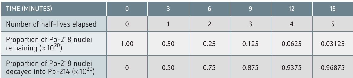
Notice how after 5 half-lives (15 minutes), only about 3% of the original polonium-218 nuclei remain. More than 96% have decayed into lead-214.

chatImportant

After approximately 5 half-lives, a radioactive sample has less than 5% of its original radioactivity remaining. This is an important principle for understanding when radioactive materials become relatively safe.

Mathematical relationships in radioactive decay

The exponential decay formula

For a sample containing $N_0$ radioactive particles initially, the number of particles $N_t$ remaining after time $t$ follows an exponential decay pattern:

$N_t = N_0 e^{-\lambda t}$

where:

$N_t$ = number of radioactive nuclei remaining at time $t$
$N_0$ = initial number of radioactive nuclei
$\lambda$ = decay constant (measured in $\text{s}^{-1}$ )
$t$ = time elapsed (measured in seconds)
$e$ = mathematical constant (approximately 2.718)

chatImportant

This formula shows that radioactive decay follows an exponential pattern, not a linear one. The sample doesn't decrease by the same amount each second; instead, it decreases by the same fraction or percentage each second.

The decay constant

The decay constant ( $\lambda$ ) is a number that characterises how quickly a particular radioactive isotope decays. Each isotope has its own specific decay constant. A larger decay constant means faster decay.

The decay constant is related to half-life by the formula:

$\lambda = \frac{\ln 2}{t_{1/2}}$

where:

$\lambda$ = decay constant ( $\text{s}^{-1}$ )
$\ln 2$ = natural logarithm of 2 (approximately 0.693)
$t_{1/2}$ = half-life (in seconds)

infoNote

This relationship allows you to convert between half-life and decay constant. If you know one, you can calculate the other. Remember: "Lambda links to ln2" - the decay constant is always connected to the natural logarithm of 2 divided by the half-life.

The half-life formula

An alternative formula useful for calculations involving whole numbers of half-lives is:

$N_t = N_0 \left(\frac{1}{2}\right)^n$

where:

$n$ = number of half-lives elapsed (a whole number)

This formula is particularly helpful for quick calculations when the time elapsed is a simple multiple of the half-life.

Worked examples

lightbulbExample

Worked Example 1: Finding the decay constant from percentage remaining

Suppose after 300 years, only 10% of the original unstable nuclei remain in a radioactive sample. We can find the decay constant as follows.

Step-by-step solution:

Step 1: Convert the time to SI units (seconds): $t = 300 \times 365 \times 24 \times 60 \times 60 = 9.46 \times 10^9 \text{ s}$

Step 2: Express the remaining fraction as a decimal: $\frac{N_t}{N_0} = 10\% = 0.1$

Step 3: Use the exponential decay formula and rearrange: $N_t = N_0 e^{-\lambda t}$ $\frac{N_t}{N_0} = e^{-\lambda t}$ $0.1 = e^{-\lambda \times 9.46 \times 10^9}$

Step 4: Take the natural logarithm of both sides: $\ln(0.1) = -\lambda \times 9.46 \times 10^9$

Step 5: Solve for $\lambda$ : $\lambda = \frac{-\ln(0.1)}{9.46 \times 10^9} = 2.43 \times 10^{-10} \text{ s}^{-1}$

lightbulbExample

Worked Example 2: Finding the decay constant from half-life

If a radioactive sample has a half-life of 6.00 hours, we can find its decay constant.

Step-by-step solution:

Step 1: Convert the half-life to seconds: $t_{1/2} = 6.00 \times 60 \times 60 = 2.16 \times 10^4 \text{ s}$

Step 2: Apply the decay constant formula: $\lambda = \frac{\ln 2}{t_{1/2}} = \frac{\ln 2}{2.16 \times 10^4}$

Step 3: Calculate the result: $\lambda = 3.21 \times 10^{-5} \text{ s}^{-1}$

lightbulbExample

Worked Example 3: Finding half-life from decay constant

If a radioactive sample has a decay constant of $3.4 \times 10^{-9} \text{ s}^{-1}$ , we can determine its half-life.

Step-by-step solution:

Step 1: Start with the relationship between decay constant and half-life: $\lambda = \frac{\ln 2}{t_{1/2}}$

Step 2: Rearrange to solve for half-life: $t_{1/2} = \frac{\ln 2}{\lambda}$

Step 3: Substitute the known value: $t_{1/2} = \frac{\ln 2}{3.4 \times 10^{-9}} = 2.0 \times 10^7 \text{ s}$

lightbulbExample

Worked Example 4: Finding percentage remaining after multiple half-lives

What percentage of nuclei remains undecayed after 40 days if the radioactive sample has a half-life of 8 days?

Step-by-step solution:

Step 1: Calculate the number of half-lives: $n = \frac{40}{8} = 5$

Step 2: Use the half-life formula with $N_0 = 1$ : $N_t = N_0 \left(\frac{1}{2}\right)^n = \left(\frac{1}{2}\right)^5$

Step 3: Calculate the result: $N_t = 0.031$

Step 4: Express as a percentage: $0.031 \times 100\% = 3.1\%$

This shows that after 5 half-lives, only about 3% of the original radioactive nuclei remain.

Practical applications

Medical uses of radioisotopes

The concept of half-life is crucial in medical applications of radioactive materials. When radioisotopes are injected into patients for diagnostic scans, it's essential that they have short half-lives. This ensures that the radioactivity diminishes quickly after the scan is complete, minimising the patient's exposure to radiation.

infoNote

Medical Example: Technetium-99m

Technetium-99m (Tc-99m) is commonly used in medical imaging and has a half-life of only 6 hours. After 24 hours (which equals 4 half-lives), the radioactivity has decreased to just 6.25% of the original level. This rapid decrease makes it much safer for medical use.

Investigation: Simulating radioactive decay

Understanding radioactive decay becomes clearer through practical simulation. This investigation uses counters or coins to model the random decay process.

infoNote

Aim: To simulate the random decay and half-life of a radioactive nuclide.

Materials needed:

80 small counters with distinguishable sides (or coins)
A bag or cup
Gloves for handling

Method:

Designate one side of the counters as "decayed" and the other as "not decayed"
Place all counters in the bag and shake thoroughly
Pour counters onto a table
Remove and count all "decayed" counters
Count and record the remaining "not decayed" counters
Return only the "not decayed" counters to the bag
Repeat the process until one or no counters remain

Analysis:

By plotting the number of remaining counters against the number of trials (throws), you should observe an exponential decay curve. From this graph, you can determine the half-life of the counters - the number of throws required for half the counters to be removed.

chatImportant

Why this simulation works:

This simulation models radioactive decay because:

Each counter has an equal, random chance of showing either side when poured (modelling the random nature of decay)
In each trial, approximately half the counters will "decay" (be removed)
The process continues exponentially, just like real radioactive decay

This hands-on activity demonstrates that whilst individual decay events are random and unpredictable, the overall pattern for large numbers follows a predictable exponential decrease.

Important exam tips

chatImportant

When solving problems involving radioactive decay:

Always convert time to seconds when using the formulas. The decay constant $\lambda$ has units of $\text{s}^{-1}$ , so time must be in seconds.
Choose the right formula: Use $N_t = N_0(1/2)^n$ when dealing with whole numbers of half-lives. Use $N_t = N_0 e^{-\lambda t}$ for any time period.
Remember your calculator functions: You'll need the natural logarithm (ln) and exponential ( $e^x$ ) functions for these calculations.
Check your significant figures: Express your final answer with the appropriate number of significant figures based on the data given.
Units matter: Always include units in your final answer, particularly for decay constant ( $\text{s}^{-1}$ ) and half-life (seconds, hours, days, or years as appropriate).

Remember!

bookmarkSummary

Key Points to Remember:

Radioactive decay is random - you cannot predict when any individual nucleus will decay, but you can predict the behaviour of large samples.
Half-life is the time for half the nuclei to decay - each radioactive isotope has its own unique half-life value.
Three key formulas to remember:
- $N_t = N_0 e^{-\lambda t}$ for exponential decay
- $\lambda = \frac{\ln 2}{t_{1/2}}$ linking decay constant and half-life
- $N_t = N_0(1/2)^n$ for whole numbers of half-lives
After 5 half-lives, less than 5% remains - this is useful for estimating when a radioactive sample has effectively decayed.
Medical radioisotopes need short half-lives - this ensures patient safety by reducing radiation exposure time.

Decay and Half-Life (HSC SSCE Physics): Revision Notes