Fitting a Linear Model to the Data Revision Notes for VCE SSCE General Mathematics

Fitting a Linear Model to the Data

Introduction to linear modeling

When we observe a linear relationship between two numerical variables on a scatterplot, we can take the analysis further by creating a linear model. This involves fitting a straight line to the data and determining its equation. The resulting line helps us better understand the relationship between variables and enables us to make predictions about future values.

The process of fitting a straight line to data showing a linear association is called linear regression. The line itself is known as the regression line or line of good fit.

infoNote

The equation of any regression line follows the standard form:

$y = a + bx$

where:

$a$ represents the $y$ -intercept (where the line crosses the vertical axis)
$b$ represents the slope (the steepness of the line)

Fitting a line 'by eye'

The most straightforward approach to fitting a linear model is the visual method, sometimes called fitting by eye. This involves using a ruler to draw a straight line on the scatterplot that appears to balance the data points evenly on both sides. Ideally, the line should have roughly equal numbers of points above and below it.

Once you have drawn this line on your scatterplot, you can determine its equation using techniques for finding the equation of a straight line.

Method 1: Using the intercept and slope

This method involves identifying the $y$ -intercept directly from the graph and calculating the slope using two convenient points on the line.

Steps:

Read the $y$ -intercept ( $a$ ) from where the line crosses the vertical axis
Calculate the slope ( $b$ ) using:

$b = \frac{\text{rise}}{\text{run}} = \frac{y_2 - y_1}{x_2 - x_1}$

Write the equation as $y = a + bx$

lightbulbExample

Worked Example: Finding the Line Equation Using Intercept and Slope

A line has been fitted by eye to data showing the velocity of an accelerating car over time.

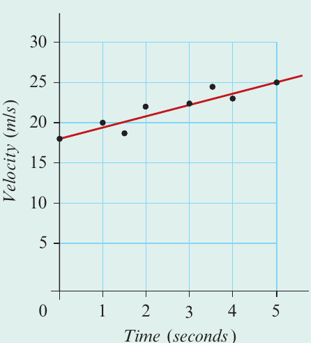
To find the equation:

The $y$ -intercept: $a \approx 18$ m/s (reading from the graph where time = 0)
The slope: Using points $(0, 18)$ and $(5, 25)$ :

$b = \frac{25 - 18}{5 - 0} = \frac{7}{5} = 1.4$

Therefore: $\text{velocity} = 18 + 1.4 \times \text{time}$

Method 2: Using two points on the line

This alternative method uses the coordinates of two clear points on the fitted line.

Steps:

Identify two points on the line where coordinates can be read easily from the graph
Calculate the slope ( $b$ ) using: $b = \frac{y_2 - y_1}{x_2 - x_1}$
Substitute one point's coordinates into $y = a + bx$ and solve for $a$
Write the final equation using the actual variable names

lightbulbExample

Worked Example: Finding the Line Equation Using Two Points

A line has been fitted to a scatterplot showing student-staff ratios in primary versus secondary education.

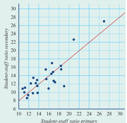
Working through the steps:

Two suitable points on the line: $(14, 12)$ and $(30, 28)$
Calculate slope:

$b = \frac{28 - 12}{30 - 14} = \frac{16}{16} = 1.0$

Find intercept using point $(14, 12)$ :

$12 = a + 1 \times 14$

$a = 12 - 14 = -2$

Final equation:

$\text{student-staff ratio secondary} = -2 + 1 \times \text{student-staff ratio primary}$

Understanding residuals

When we fit a line to data, most points will not lie exactly on the line. The vertical distance between each actual data point and the fitted line is called a residual.

infoNote

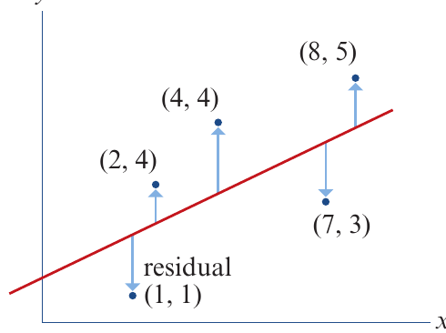
Residuals can be:

Positive when the actual data point lies above the line
Negative when the actual data point lies below the line

These residuals are important because they measure how well our line fits the data. Smaller residuals indicate a better fit.

The least squares method

While fitting a line by eye is simple, a more precise mathematical approach is the least squares method. This technique finds the single best line for the data based on a clear mathematical criterion.

How the method works

The least squares method finds the line that minimises the sum of the squared residuals. Here's why we square the residuals:

Some residuals are positive (points above the line)
Some residuals are negative (points below the line)
If we simply added residuals together, positive and negative values would cancel out
By squaring each residual first, all values become positive
We can then add them together meaningfully
The line that makes this sum as small as possible is our best fit

The name "least squares" comes from finding the line with the least value for the sum of squared residuals.

Formulas for the least squares line

The least squares regression line has equation $y = a + bx$ , where the slope and intercept are calculated using these formulas:

Slope:

$b = r \frac{s_y}{s_x}$

Intercept:

$a = \bar{y} - b\bar{x}$

where:

$r$ is the correlation coefficient
$s_x$ and $s_y$ are the standard deviations of $x$ and $y$
$\bar{x}$ and $\bar{y}$ are the mean values of $x$ and $y$

chatImportant

Always calculate the slope ( $b$ ) first, as you need it to find the intercept ( $a$ ).

Assumptions for using least squares

Before applying the least squares method, check that:

Both variables are numerical (not categorical)
The association appears linear (not curved) on the scatterplot

These are the same assumptions required for calculating Pearson's correlation coefficient.

Worked example: Calculating the least squares line

lightbulbExample

Worked Example: Calculating the Least Squares Line

Find the equation of the least squares regression line when:

$r = 0.600, \quad s_x = 9.80, \quad s_y = 5.40, \quad \bar{x} = 165.0, \quad \bar{y} = 62.3$

Solution:

Calculate the slope:

$b = r \frac{s_y}{s_x} = 0.600 \times \frac{5.40}{9.80} = 0.3306$

Calculate the intercept:

$a = \bar{y} - b\bar{x} = 62.3 - 0.3306 \times 165.0 = 7.751$

Write the equation (rounded to 3 significant figures):

$y = 7.75 + 0.331x$

chatImportant

Exam tip: When performing these calculations, work with more decimal places than required and only round your final answer to avoid rounding errors accumulating.

Using technology to find the least squares line

Modern calculators can determine the least squares regression line directly from your data. Both TI-Nspire CAS and ClassPad calculators have built-in functions for this purpose.

General process (all calculators)

Enter your data into two lists or columns
Identify which variable is explanatory (independent, on $x$ -axis) and which is response (dependent, on $y$ -axis)
Create a scatterplot
Use the regression function to fit a linear model
The calculator displays the equation and correlation coefficient

Example using calculator functions

lightbulbExample

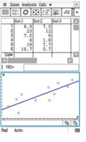
Worked Example: Using Technology for Linear Regression

For the income and CO₂ emissions data:

Income (\$'000)	8.9	23.0	7.5	8.0	18.0	16.7	5.2	12.8	19.1	16.4	21.7
CO₂ (tonnes)	7.5	12.0	6.0	1.8	7.7	5.7	3.8	5.7	11.0	9.7	9.9

The calculator produces:

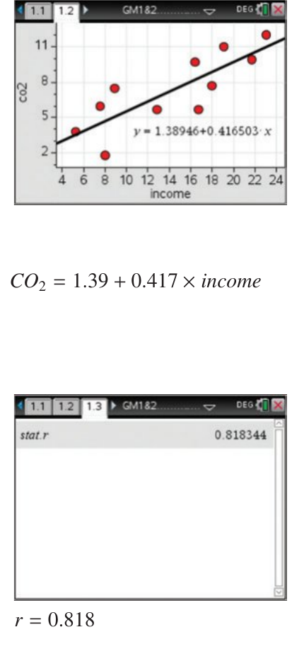
The output shows:

Regression equation: $y = 1.389 + 0.417x$
Correlation coefficient: $r = 0.818$

In terms of the actual variables:

$\text{CO}_2 = 1.39 + 0.417 \times \text{income}$

This tells us that for every \$1,000 increase in income, CO₂ emissions increase by approximately 0.417 tonnes on average.

chatImportant

Exam tip: Even when using a calculator, always write your final equation using the actual variable names from the question, not just $x$ and $y$ . This demonstrates understanding of what the equation represents.

Interpreting the regression line

When you have found the equation of the regression line:

The slope tells you how much the response variable changes for each unit increase in the explanatory variable
The intercept gives the predicted value of the response variable when the explanatory variable equals zero (though this may not always be meaningful in context)
The correlation coefficient indicates the strength and direction of the linear relationship

bookmarkSummary

Key Points to Remember:

Linear regression creates a mathematical model of the linear relationship between two numerical variables
The regression line equation is $y = a + bx$ , where $a$ is the intercept and $b$ is the slope
Fitting by eye is a simple visual method—draw a line that balances the points
Residuals are the vertical distances between data points and the fitted line
The least squares method finds the line that minimises the sum of squared residuals—this is the best mathematical fit
Always calculate slope first: $b = r(s_y/s_x)$ , then intercept: $a = \bar{y} - b\bar{x}$
Calculators can determine the least squares line efficiently, but always express the final equation using the actual variable names from your context

Fitting a Linear Model to the Data (VCE SSCE General Mathematics): Revision Notes