Biodiversity (AQA A-Level Biology): Revision Notes
Quantitative Investigations of Variation
Understanding variation and measurement challenges
Living organisms show remarkable diversity both between and within species. Interspecific variation refers to differences between different species, while intraspecific variation describes differences between individuals of the same species. Even identical twins with the same DNA show variation due to their different experiences throughout life.
Measuring biological variation presents unique challenges for scientists. Unlike measuring non-living objects, biologists cannot simply take a single measurement to characterise a population. For example, you cannot determine the height of all buttercups or count red blood cells in human blood from just one measurement.
This fundamental challenge in biology is why sampling becomes essential - we need multiple measurements to understand the true nature of biological populations and their characteristics.
This is why biologists must take samples - collections of measurements from individuals selected from the population being studied.
Random sampling principles
Sampling involves taking measurements from individuals selected from the population under investigation. For these measurements to be reliable and representative of the entire population, the sampling process must be carefully designed.
The key principle is that samples should be representative of the population as a whole. However, several factors can compromise this representativeness:
Common Sources of Sampling Problems:
Sampling bias occurs when the selection process is biassed, either deliberately or unintentionally. Examples include:
- Choosing samples from convenient but unrepresentative locations (such as only sampling buttercups from dry areas rather than muddy ones)
- Avoiding certain areas due to practical difficulties (like areas rich in nettles or covered in cow dung)
Chance can also affect representativeness. Even with unbiased sampling methods, the individuals chosen might not represent the population accurately by pure chance.
Implementing random sampling
The most effective way to prevent sampling bias is to eliminate human involvement in choosing samples through random sampling. One systematic method involves:
Systematic Random Sampling Method:
- Dividing the study area into a numbered grid using measuring tapes at right angles
- Using random numbers (from tables or computer-generated) to obtain coordinate pairs
- Taking samples at the intersection points of these randomly selected coordinates
This method ensures that human preferences and unconscious biases don't influence which samples are selected.
Minimising chance effects
While random sampling reduces bias, chance effects cannot be completely eliminated. However, their influence can be minimised through:
- Using large sample sizes: The probability that chance will influence results decreases as sample size increases. Sampling 500 individuals gives much more reliable data than sampling only five individuals.
- Statistical analysis of collected data: Mathematical tests can determine whether observed variation is likely due to chance or represents genuine biological differences. These tests help scientists decide if their results are statistically significant.
The normal distribution curve
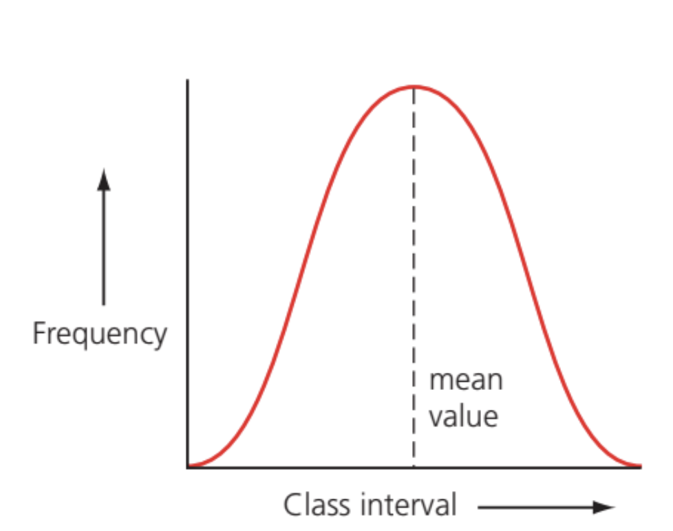
When continuous variation data is plotted graphically, it typically produces a normal distribution curve - a symmetrical, bell-shaped pattern. This curve is characteristic of features like human height, where most individuals cluster around an average value with fewer individuals at the extremes.
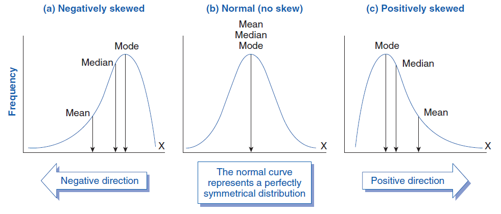
In a normal distribution, the curve is perfectly symmetrical, meaning the mean, mode, and median all have the same value and occur at the peak of the curve.
Sometimes the curve becomes skewed, meaning it shifts slightly to one side, creating asymmetry. In skewed distributions, the mean, mode, and median have different values, unlike in normal distributions where they coincide.
Measures of central tendency
Three key statistical measures describe the central or typical value in a data set:
- Mean (arithmetic mean): The sum of all sampled values divided by the number of items.
This provides an average value and is particularly useful for comparing different samples. However, it gives no information about the range or spread of values within the sample.
- Mode: The single value that occurs most frequently in the sample. In some data sets, there may be more than one mode if multiple values occur with equal highest frequency.
- Median: The central or middle value when all measurements are arranged in ascending order. For an odd number of values, this is the middle value. For an even number of values, it's the average of the two middle values.
Standard deviation
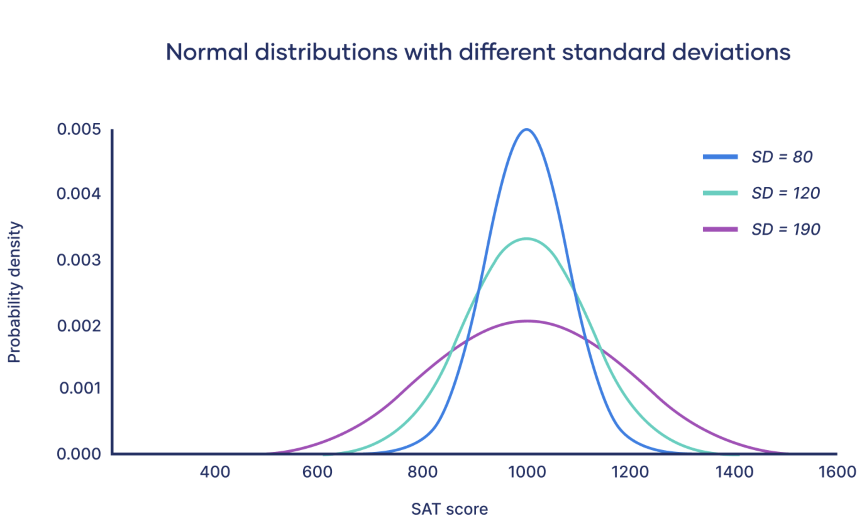
Standard deviation is a measure of how widely data values are spread around the mean. It provides crucial information about the variability within a sample.
A small standard deviation indicates that most values cluster closely around the mean (little variety), while a large standard deviation shows that values are more widely spread (high variety).
Key Statistical Facts:
In a normal distribution:
- 68% of all measurements lie within ±1.0 standard deviation of the mean
- 95% of all measurements lie within approximately ±2.0 standard deviations of the mean
The point of inflexion on the curve occurs at one standard deviation from the mean, where the curve changes from convex to concave.
Calculating standard deviation
The formula for standard deviation appears complex but becomes manageable when calculated step by step:
Where:
- = sum of
- = measured value from the sample
- = mean value
- = total number of values in the sample
Step-by-step calculation process:
- Calculate the mean value () by adding all measurements and dividing by the number of items
- Subtract the mean from each individual measured value
- Square all these differences - remember to square both positive and negative values
- Add all the squared values together
- Divide by where is the number of measurements
- Take the square root to return to the original units
Worked Example: Standard Deviation Calculation
For values 4, 1, 2, 3, 5, 0:
Step 1: Calculate mean =
Step 2: Find differences from mean:
- 4 - 2.5 = +1.5
- 1 - 2.5 = -1.5
- 2 - 2.5 = -0.5
- 3 - 2.5 = +0.5
- 5 - 2.5 = +2.5
- 0 - 2.5 = -2.5
Step 3: Square the differences:
Step 4: Sum = 2.25 + 2.25 + 0.25 + 0.25 + 6.25 + 6.25 = 17.5
Step 5: Divide by :
Step 6: Take square root:
Significant figures and calculations
When using calculators for standard deviation calculations, you'll often get very long decimal answers. The significance of digits decreases from left to right, so it's normal practice to round answers to an appropriate number of significant figures.
Best Practice for Significant Figures:
Always follow any specific instructions about significant figures in exam questions. When no guidance is given, use the same number of significant figures as the original data. For calculations that will be used in subsequent steps, avoid rounding until the final answer to maintain accuracy.
Key Points to Remember:
- Random sampling eliminates bias by removing human choice from sample selection, making data more representative of the population
- Large sample sizes reduce chance effects and increase the reliability of results
- Normal distribution curves are symmetrical with mean, mode, and median having the same value
- Standard deviation measures data spread - small values indicate clustered data, large values indicate widely spread data
- Statistical analysis helps distinguish between variation due to chance and variation with biological significance