Aggregate Demand and Supply Analysis Revision Notes for AQA A-Level Economics

Aggregate Demand and Supply Analysis

Introduction to the AD/AS model

Over the past 40 years, the AD/AS model has become the main theoretical framework that economists use to analyse macroeconomic issues. This model helps us understand how changes in aggregate demand and aggregate supply affect the economy's overall performance, including real output, employment levels, and the price level.

infoNote

The model addresses a fundamental question in economics: when government uses fiscal or monetary policy to increase aggregate demand, will this lead to higher real output and more jobs, or will it simply cause the price level to rise? The answer depends largely on supply-side factors, which are represented by the shape of the aggregate supply curve in both the short run and the long run.

Understanding aggregate demand

What is aggregate demand?

Aggregate demand (AD) represents the total planned spending on goods and services produced within the economy during a specific time period, typically measured over a year. It encompasses spending from all sectors of the economy: households, firms, the government sector, and the overseas sector.

The aggregate demand equation

The components of aggregate demand are expressed in this equation:

$AD = C + I + G + (X - M)$

Where:

C = Consumption (household spending on goods and services)
I = Investment (business spending on capital goods)
G = Government spending (public sector expenditure)
X = Exports (foreign spending on domestic goods)
M = Imports (domestic spending on foreign goods)

Note that exports minus imports $(X - M)$ represents net exports, which can be positive (trade surplus) or negative (trade deficit).

The AD curve

The AD curve illustrates the relationship between the price level in the economy and the quantity of real output demanded. The curve slopes downwards from left to right, showing an inverse relationship between these two variables.

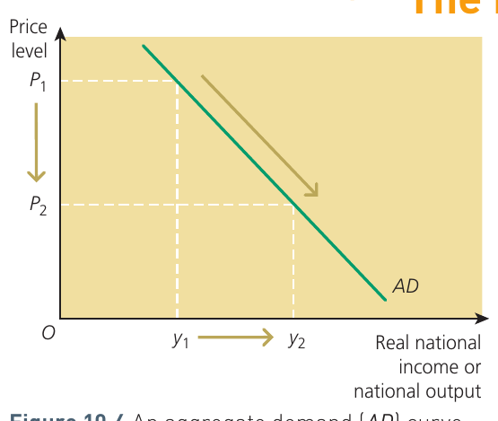
Why does the AD curve slope downwards?

When the price level falls in the economy, several things happen:

Exports become more price competitive in international markets
Foreign buyers are likely to purchase more of the country's goods and services
This leads to increased spending overall
Total aggregate demand therefore rises

At lower price levels, the quantity of real output demanded is higher. Conversely, at higher price levels, the quantity of real output demanded is lower.

chatImportant

Important distinction: Although the AD curve slopes downwards like a microeconomic demand curve, the reasons for this slope are different. In microeconomics, we explain the downward slope through substitution and income effects for individual goods. In macroeconomics, the downward slope reflects how changes in the overall price level affect international competitiveness and total national spending.

Movements along versus shifts of the AD curve

Understanding the difference between movements along the AD curve and shifts of the entire curve is crucial for economic analysis.

Movements along the AD curve occur when the price level changes. As the price level moves up or down, we move to a different point on the same AD curve. These movements are typically connected with changes in aggregate supply rather than changes in aggregate demand itself.

Shifts of the AD curve occur when there is a change in the value of any component of aggregate demand $(C, I, G, X, \text{ or } M)$ at any given price level. For example:

A rise in business confidence could increase investment $(I)$
A fall in interest rates could increase both consumption $(C)$ and investment $(I)$
Changes in government policy could affect government spending $(G)$
Changes in exchange rates could affect exports $(X)$ and imports $(M)$

Any of these changes would cause the entire AD curve to shift to a new position - rightwards for an increase in AD, leftwards for a decrease.

Worked example: calculating aggregate demand

Let's examine how to calculate aggregate demand using real data. The table below shows the components of aggregate demand for an economy in 2022 and 2023:

lightbulbExample

Worked Example: Calculating Aggregate Demand

Year	Government and private consumption expenditure	Government and private investment expenditure	Exports	Imports
2022	1,000	150	300	200
2023	1,200	170	250	220

Question (a): What was the change in aggregate demand between 2022 and 2023?

Using the aggregate demand equation: $AD = C + I + G + (X - M)$

For 2022:

$AD = £1,000bn + £150bn + £300bn - £200bn = £1,250bn$

For 2023:

$AD = £1,200bn + £170bn + £250bn - £220bn = £1,400bn$

Therefore, between 2022 and 2023, aggregate demand increased by £150 billion.

Question (b): What was the change in net export demand between 2022 and 2023?

In 2022, net export demand $(X - M)$ was $£300bn - £200bn = £100$ billion.

In 2023, net export demand $(X - M)$ was $£250bn - £220bn = £30$ billion.

There was a balance of trade surplus in both years (exports exceeded imports). However, the trade surplus fell by £70 billion between 2022 and 2023.

infoNote

Study tip: Make sure you don't confuse aggregate demand with national expenditure. Both are macroeconomic concepts related to demand in the whole economy. However, aggregate demand measures planned spending, whereas national expenditure measures realised or actual spending that has already taken place.

Understanding aggregate supply

What is aggregate supply?

Aggregate supply (AS) represents the level of real national output that producers are willing and able to supply at different average price levels. In the short run, the AS curve slopes upward, showing that firms will supply more output when prices are higher.

The short-run AS curve

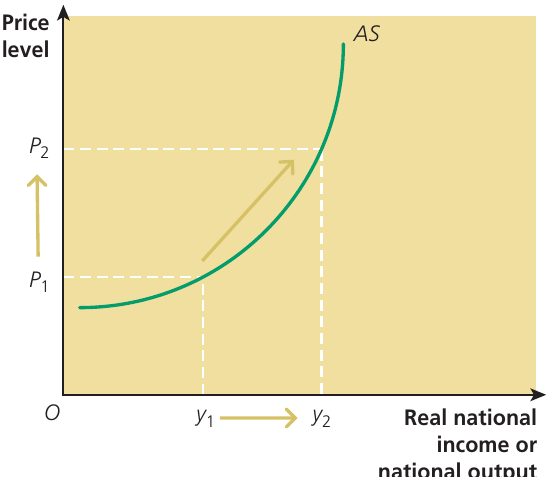
The upward slope of the short-run aggregate supply (SRAS) curve is explained by two key microeconomic assumptions about how firms behave:

All firms aim to maximise profits
In the short run, the cost of producing extra units of output increases as firms produce more

Consider what happens at different price levels. At a lower average price level $(P_1)$ , the economy's firms are willing to produce and sell a certain level of output $(y_1)$ . To persuade these firms to produce more output $(y_2)$ , the price level must rise to $P_2$ .

Why must prices rise to increase supply?

Higher prices are needed to create the higher sales revenues necessary to offset the increased production costs that firms face when they expand output. Without this price increase, profit-maximising firms would not voluntarily choose to supply more output. The curve becomes steeper at higher output levels because production costs rise more rapidly as firms approach full capacity.

Movements along versus shifts of the AS curve

Just like with the AD curve, it's essential to distinguish between movements along the AS curve and shifts of the entire curve.

Movements along the AS curve occur when the price level changes. These represent changes in the quantity of output supplied in response to price changes, with all other factors held constant.

Shifts of the AS curve occur when factors other than the price level change. The AS curve is constructed assuming all determinants of aggregate supply apart from price remain unchanged. If any of these other determinants change, the AS curve shifts to a new position.

infoNote

Factors that can shift the AS curve include:

Changes in wage rates
Changes in productivity
Changes in raw material costs
Changes in business taxes
Changes in technology

For example, a fall in wage rates or an increase in productivity would decrease production costs, causing the AS curve to shift rightward (an increase in aggregate supply). Conversely, a rise in raw material costs would increase production costs, shifting the AS curve leftward (a decrease in aggregate supply).

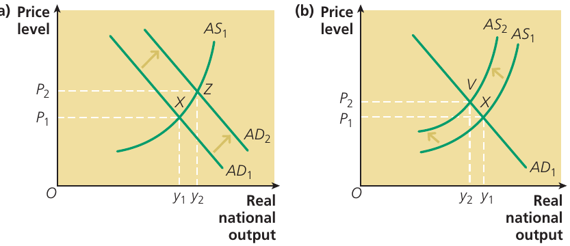
The diagram above illustrates both types of changes. Panel (a) shows a rightward shift of the AD curve from $AD_1$ to $AD_2$ , leading to a movement along the AS curve. Panel (b) shows a leftward shift of the AS curve from $AS_1$ to $AS_2$ , leading to a movement along the AD curve.

chatImportant

Study tip: Remember the key difference - an increase or decrease in AD is shown as a shift in the AD curve, which then leads to a movement along the AS curve (either an expansion or contraction of AS). Similarly, an increase or decrease in AS is shown as a shift in the AS curve, which leads to a movement along the AD curve (either an expansion or contraction of AD). Don't confuse shifts in curves with movements along curves.

Long-run aggregate supply (LRAS)

Understanding the LRAS curve

The aggregate supply curves discussed so far have been short-run aggregate supply (SRAS) curves. We now introduce a different concept: the economy's long-run aggregate supply (LRAS) curve.

Long-run aggregate supply represents the real output that can be supplied when the economy is operating on its production possibility frontier. This is the maximum level of output the economy can produce when all available factors of production are employed and producing at their normal capacity.

Why is the LRAS curve vertical?

The LRAS curve is depicted as a vertical line, which has important implications for economic analysis.

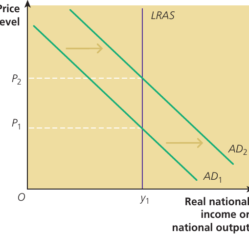
In the short run, aggregate supply depends on the average price level in the economy. When other factors remain constant, firms will only supply more output if prices rise. However, in the long run, aggregate supply is not influenced by the price level. Instead, long-run supply reflects the economy's productive capacity - it represents the maximum output the economy can produce when operating on its production possibility frontier.

The diagram above shows what happens when aggregate demand increases from $AD_1$ to $AD_2$ when the economy is already at full capacity (on the LRAS curve). Since there is no spare capacity or idle resources, output cannot increase beyond $y_1$ . The increase in aggregate demand simply causes the price level to rise from $P_1$ to $P_2$ , resulting in inflation without any increase in real output.

LRAS and economic growth

Long-run economic growth occurs when the economy's productive capacity expands. This is represented by a rightward shift of both the production possibility frontier and the LRAS curve.

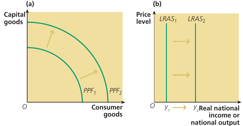
The two diagrams above illustrate the same economic concept in different ways:

Panel (a) shows an outward shift of the production possibility frontier from $PPF_1$ to $PPF_2$
Panel (b) shows a rightward shift of the LRAS curve from $LRAS_1$ to $LRAS_2$

Both represent an increase in the economy's productive capacity and potential output.

What causes the LRAS curve to shift?

infoNote

Underlying economic growth - the long-run average growth rate for a country - is determined by factors that affect the position of the economy's production possibility frontier:

Increases in the quantity of factors of production, particularly labour and capital
Improvements in the quality of factors of production, such as through education and training
Technological progress that increases productivity
Better organisation and management of resources

These factors shift both the production possibility frontier outward and the LRAS curve to the right, enabling the economy to produce more output in the long run.

infoNote

Study tip: Long-run economic growth can be shown either through an outward movement of the production possibility frontier or through a rightward shift of the LRAS curve. Short-run economic growth, by contrast, comes from an increase in AD (or occasionally an increase in SRAS), which moves the economy towards its production possibility frontier.

Macroeconomic equilibrium

Equilibrium in the AD/AS model

There are two approaches to understanding macroeconomic equilibrium, and both are important.

The first approach (covered in previous sections) views equilibrium as occurring when planned injections into the circular flow of income equal planned withdrawals from the flow. The second approach uses the AD/AS model.

In the AD/AS model, equilibrium national income occurs when the aggregate demand for real output equals the aggregate supply of real output, that is, where AD = AS.

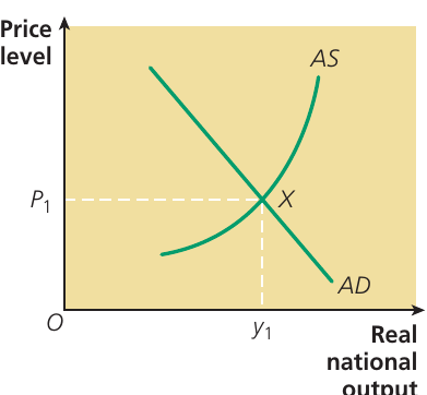
The diagram above illustrates macroeconomic equilibrium. The AD curve intersects the AS curve at point X. At this point:

The equilibrium level of real output is $y_1$
The equilibrium price level is $P_1$

At equilibrium, there is no tendency for output or the price level to change, assuming the AD and AS curves remain in their current positions. The economy is in a stable position where the quantity of output demanded equals the quantity of output supplied.

Economic shocks

What are economic shocks?

An economic shock is a sudden, unexpected event that hits the economy. Economic shocks disturb either aggregate demand (demand-side shocks), aggregate supply (supply-side shocks), or sometimes both. They can be either unfavourable or favourable for the economy.

Economic shocks have important effects because they shift either the AD curve or the AS curve (or both), causing changes in real output, employment, and the price level.

Recent economic shocks

Since 2007, several major economic shocks have affected the UK economy:

The financial crisis of 2007-08 (both demand and supply-side effects)
The UK leaving the European Union (the shock arguably occurred after the UK fully left in 2021)
The Covid-19 pandemic beginning in 2020 and continuing beyond
The war in Ukraine beginning in 2022

Some of these shocks primarily affected the demand side of the economy, some affected the supply side, and some affected both.

chatImportant

Study tip: When analysing which curve will shift in response to an economic event, consider:

AD is determined by factors affecting national spending (consumption, investment, government spending, net exports)
SRAS is determined by factors that affect costs of production and the profitability of production
LRAS is determined by the economy's productive capacity (quantity and quality of factors of production, technology)

Case study: Economic shock caused by the El Niño effect

infoNote

Background to El Niño:

Above-average ocean surface temperatures develop every three to seven years off the Pacific coast of South America and last about two years, causing major climatological changes around the world. This phenomenon is called the El Niño effect. The 2015-16 El Niño was one of the most severe events in the past 50 years and the largest since the 1997-98 El Niño that shocked global food, water, health, energy and disaster-response systems.

Climate impacts:

Economists are increasingly interested in the relationship between climate (temperature, precipitation, storms and other aspects of weather) and economic performance. The extreme weather conditions associated with El Niño can constrain the supply of rain-driven agricultural commodities, lead to higher food prices and inflation, and may trigger social unrest in countries that rely primarily on imported food.

An El Niño typically brings drought to the western Pacific (including Australia), rains to the equatorial coast of South America, and storms and hurricanes to the central Pacific. These changes in weather patterns have significant effects on agriculture, fishing and construction industries, as well as on national and global commodity prices.

Economic effects:

Different countries experience different impacts:

Australia, Chile, India, Indonesia, Japan, New Zealand and South Africa typically face a short-lived fall in economic activity in response to a typical El Niño shock
In other countries, the climate actually boosts GDP - in the USA, for example, reduced hurricanes and improved outputs of certain crops can have positive effects
Many countries experience short-term inflation pressures following an El Niño shock, as its magnitude increases with the share of food in the consumer prices index basket
Prices of energy and non-fuel commodities (goods that are identical, so are interchangeable) also rise around the world

Wider global impacts:

Climate change and global warming in sub-Saharan economies have led to severe drought and desertification, dramatically increasing the area of the Sahara desert. Several African countries are experiencing economic crisis and increasing poverty due to civil war, drought and famine. This means many people choose to emigrate in search of better economic prospects.

infoNote

Study tip: You should build up knowledge of four or five economic shocks that have affected the UK and global economies in recent years. Consider whether these are demand-side or supply-side shocks (or both).

Remember!

bookmarkSummary

Key Points to Remember:

Aggregate demand shows total planned spending in the economy and consists of four components: consumption, investment, government spending, and net exports $(AD = C + I + G + (X - M))$
The AD curve slopes downward because at lower price levels, exports become more competitive and aggregate demand increases. A change in the price level causes a movement along the AD curve, while changes in spending components cause the curve to shift
The short-run AS curve slopes upward because firms require higher prices to cover increased production costs when expanding output. Changes in production costs (wages, raw materials, productivity) cause the AS curve to shift
The LRAS curve is vertical at the economy's maximum productive capacity. It represents the output level when the economy is on its production possibility frontier. Economic growth is shown by a rightward shift of the LRAS curve
Macroeconomic equilibrium occurs where the AD and AS curves intersect (where $AD = AS$ ), determining both the equilibrium price level and real output. Economic shocks can be demand-side or supply-side events that disturb this equilibrium by shifting the AD or AS curves

Aggregate Demand and Supply Analysis (AQA A-Level Economics): Revision Notes