Determinants of Short-Run and Long-Run Aggregate Supply (AQA A-Level Economics): Revision Notes

Determinants of Short-Run and Long-Run Aggregate Supply

Introduction to aggregate supply

Aggregate supply represents the total quantity of goods and services that producers in an economy are willing and able to supply at different price levels. Understanding what determines aggregate supply is crucial for analysing how the macroeconomy works and how policy changes affect economic performance.

There are two key concepts to understand: short-run aggregate supply (SRAS) and long-run aggregate supply (LRAS). Each has different determinants, and understanding these differences is essential for A-Level Economics.

Determinants of short-run aggregate supply

Main determinants of SRAS

The short-run aggregate supply curve shows the relationship between the price level and the quantity of real output that firms are willing to supply, holding all other factors constant. Two primary factors influence the SRAS curve:

• The price level: As prices rise in the economy, firms generally find it more profitable to increase production, so they supply more output.
• Production costs: The costs that businesses face when producing goods and services, including wages, raw materials, energy, and taxation.

When we draw the SRAS curve, we assume that production costs remain unchanged. Changes in these costs will cause the entire curve to shift position.

Understanding the shape of SRAS

An important feature of SRAS curves is that they are non-linear or curved, rather than straight lines. The curve becomes steeper as it moves upward, meaning that as output increases, the price level rises more rapidly.

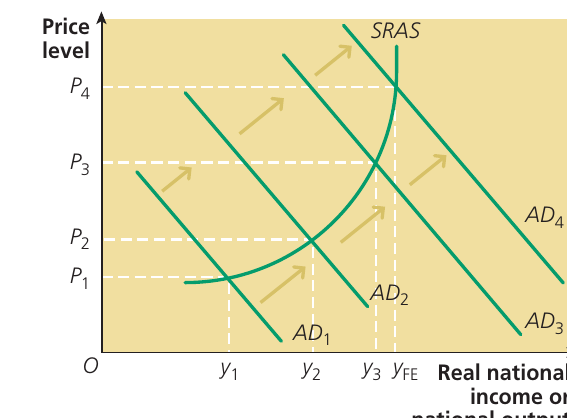
This shape has important implications for economic policy. When aggregate demand (AD) shifts along a non-linear SRAS curve:

• If AD increases when the economy is operating on a relatively flat (shallow) section of the SRAS curve, most of the effect shows up as increased real output with only a small rise in the price level. This is reflationary - boosting output without much inflation.

• If AD increases when the economy is operating on a steep section of the SRAS curve, most of the effect falls on the price level rather than real output. This is inflationary - causing rising prices with little increase in output.

• At full employment ($y_{FE}$ in the diagram), any further increase in aggregate demand can only raise the price level. The economy cannot increase output beyond full capacity, at least in the short run.

Slope versus shift of the SRAS curve

Factors causing a rightward shift in SRAS

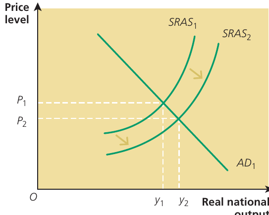
A rightward shift of the SRAS curve represents an increase in aggregate supply. At any given price level, firms are now willing to supply more output. This is beneficial for the economy as it allows for higher output with lower inflation (or even deflation).

The following factors cause the SRAS curve to shift to the right:

• A fall in businesses' costs of production: When production costs decrease, firms can profitably supply more output at each price level. This includes lower costs of imported raw materials and energy.

• A fall in unit labour costs: This can result from a fall in wage rates (though this is relatively rare) or, more commonly, from an increase in labour productivity. When workers become more productive (perhaps through better training), the cost per unit of output falls even if wages stay the same or rise slightly.

• A reduction in indirect taxes: Taxes such as VAT are imposed on firms by the government. When these taxes are reduced, production costs fall and firms can supply more.

• An increase in subsidies: Government subsidies effectively reduce production costs for firms. Greater subsidies mean firms can profitably produce more at each price level.

• Technical progress: Improvements in technology enhance the quality and productivity of capital goods. Better machinery and equipment allow firms to produce more output with the same inputs, reducing unit costs.

Factors causing a leftward shift in SRAS

A leftward shift of the SRAS curve represents a decrease in aggregate supply. At any given price level, firms are willing to supply less output. This is harmful for the economy as it tends to cause both higher inflation and lower output (sometimes called stagflation).

A leftward shift would be caused by the opposite of the factors listed above:

• Rising production costs (e.g., more expensive imported raw materials or energy)
• Increasing wage costs without corresponding productivity improvements
• Higher indirect taxes on businesses
• Reduction or removal of government subsidies
• Deterioration in technology or capital stock (rare, but can occur after disasters or conflicts)

Determinants of long-run aggregate supply

The concept of normal capacity

In the long run, aggregate supply is not influenced by the price level. Instead, long-run aggregate supply reflects the economy's production potential - the maximum level of output that the economy can sustainably produce.

Factors determining the position of the LRAS curve

The position of the LRAS curve is determined by the same factors that determine the economy's production possibility frontier. These are fundamental supply-side factors that affect the economy's capacity to produce:

1. The state of technical progress: Improvements in technology allow the economy to produce more output from the same inputs. Better production methods, more efficient machinery, and innovation all shift the LRAS curve to the right.

2. The quantities of capital and labour: The more factors of production available in the economy, the more it can produce. This includes:

• The size and quality of the capital stock (machinery, equipment, infrastructure)
• The size and skills of the labour force

3. The mobility of factors of production, particularly labour: If workers can easily move between jobs, industries, and locations, the economy can allocate resources more efficiently and produce more. Barriers to mobility (such as poor transport, housing shortages, or lack of transferable skills) reduce productive potential.

4. The productivity of the factors of production, particularly labour productivity: More productive workers generate more output per hour worked. Productivity improvements come from better education and training, better capital equipment, and improved work organisation.

5. People's attitudes to hard work: Cultural attitudes towards work, leisure, and effort can affect how hard people work and how much the economy produces.

6. Personal enterprise, particularly among entrepreneurs: The willingness of individuals to take risks, start businesses, and innovate is crucial for economic growth. Risk-taking entrepreneurs drive innovation and efficiency improvements that shift LRAS to the right.

7. Economic incentives: The existence of appropriate incentives affects how hard people work and how much they invest. This includes the tax system, welfare benefits, and the rewards for effort and risk-taking.

8. The institutional structure of the economy: This involves factors such as:

• The rule of law (protecting property rights and enforcing contracts)
• The efficiency of the banking system (providing finance to businesses)
• The quality of contract law

Alternative views of long-run aggregate supply

The vertical (free-market) LRAS curve

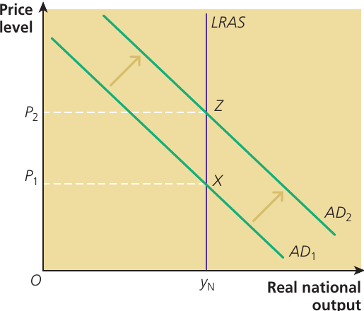
The most common representation of LRAS is as a vertical line. This vertical shape reflects the view that, in the long run, the economy operates at or close to its normal capacity, regardless of the price level.

This view is commonly associated with free-market economists who believe that:

• Markets function competitively and efficiently
• The economy naturally tends towards full employment
• In the short run, real output may be influenced by the price level, but in the long run, aggregate supply is determined by maximum normal production capacity
• The position of the vertical LRAS curve is determined by the productive capacity factors listed above

When drawn vertically, the LRAS curve shows that changes in aggregate demand affect only the price level in the long run, not real output. The economy always returns to producing at its natural capacity level.

The Keynesian aggregate supply curve

An alternative view of long-run aggregate supply was developed by the economist John Maynard Keynes during the Great Depression of the 1930s. Keynes argued that the economy could settle into an under-full-employment equilibrium for prolonged periods.

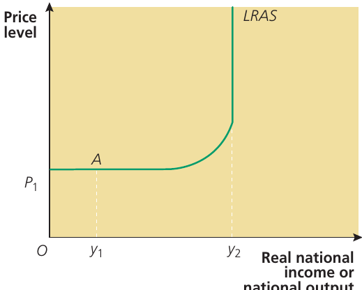
The Keynesian LRAS curve has a distinctive inverted L-shape (sometimes called a hockey stick shape):

Horizontal section: At low levels of output (such as point A on the diagram, where output is $y_1$), the curve is horizontal at price level $P_1$. This represents a depressed economy with significant spare capacity and high unemployment. In this situation, Keynes believed that:

• Firms would fail to adjust wages and prices automatically
• The economy could remain stuck with large amounts of spare capacity
• Market forces alone would not achieve full employment

Upward-sloping section: As output increases towards full capacity, the curve begins to slope upward. This reflects increasing resource constraints as the economy approaches full employment.

Vertical section: Eventually, when maximum normal capacity is achieved, the LRAS curve becomes vertical, just like the free-market LRAS curve. At this point, the economy cannot produce more output, so increases in aggregate demand only raise prices.

Temporary production above normal capacity

Even when producing at normal capacity, the economy may still be capable of temporarily producing a higher level of real output than the normal capacity level.

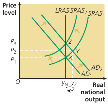
Consider an economy initially in macroeconomic equilibrium at point X, where $AD_1$ intersects both $SRAS_1$ and the LRAS curves. The economy is producing at its normal capacity level $y_n$.

If aggregate demand increases (perhaps through expansionary monetary policy lowering interest rates), AD shifts rightward to $AD_2$. This brings about a new short-run equilibrium at point Y. In this new equilibrium, real output has risen to $y_2$, which is above the normal capacity level of output.

However, this level of output - where the economy is producing above its production potential - cannot be sustained unless the LRAS curve itself shifts rightwards. Here's why:

At $y_2$, there are shortages of labour and other factors of production because the economy is operating beyond its sustainable capacity. Excess demand in labour and factor markets leads to rising factor prices. To persuade workers to supply the extra labour needed to produce $y_2$, given that the price level has risen to $P_2$, money wages must also rise.

As soon as wages rise, the SRAS curve shifts upward or leftward (to $SRAS_2$). The backward-bending curved arrow lying along the horizontal axis shows real output falling back from $y_2$ to the normal capacity level of output at $y_n$, located below point Z on the diagram.

Components of aggregate demand

To understand the context of aggregate supply, it is helpful to see how aggregate demand is composed:

Component	£bn at 2020 prices	% change in the year 2022/23
Household consumption	1,048	4.0
Investment	306	5.2
Government spending	292	3.4
Exports of goods and services	496	2.6
Imports of goods and services	570	7.1

This table shows the main components of aggregate demand in the UK economy. All components can shift the AD curve, but remember that imports are a leakage from the circular flow. Changes in any of these components can lead to movements along the SRAS curve or, if they affect production capacity, shifts in the LRAS curve.

Remember!