Price Elasticity of Supply (AQA A-Level Economics): Revision Notes

Price Elasticity of Supply

What is price elasticity of supply?

Price elasticity of supply (PES) shows how responsive the quantity supplied of a good is to changes in its price. When the price of a product changes, suppliers may be able to adjust their output quickly, or they may find it difficult to respond. PES helps us measure this responsiveness.

The formula for price elasticity of supply

We calculate PES using the following formula:

$\text{PES} = \frac{\text{percentage change in quantity supplied}}{\text{percentage change in price}}$

This formula tells us the proportional relationship between price changes and quantity supplied. For example, if a 10% increase in price leads to a 20% increase in quantity supplied, the PES would be 2.0.

Types of supply elasticity

Supply can have varying degrees of elasticity. Understanding these different types helps us analyse how different markets and industries respond to price changes.

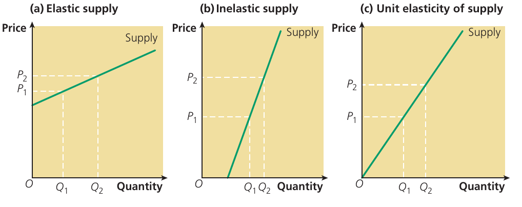
Elastic supply (PES > 1)

When supply is elastic, the percentage change in quantity supplied is greater than the percentage change in price. A small price increase leads to a proportionally larger increase in the quantity supplied.

Inelastic supply (PES < 1)

When supply is inelastic, the percentage change in quantity supplied is smaller than the percentage change in price. Even significant price increases result in only modest increases in quantity supplied.

For instance, if price rises by 10% but quantity supplied only increases by 4%, PES = 0.4, indicating inelastic supply. Firms find it difficult to adjust their output levels quickly.

Unit elasticity of supply (PES = 1)

Unit elasticity occurs when the percentage change in quantity supplied exactly equals the percentage change in price. A 10% price rise leads to exactly a 10% increase in quantity supplied.

Understanding linear supply curves and elasticity

The position and shape of supply curves tell us important information about elasticity. We must be careful not to confuse the slope of a supply curve with its elasticity - these are different concepts.

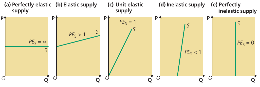
The five key linear supply curves

Perfectly elastic supply (PES = ∞): The supply curve is horizontal. Suppliers will provide any quantity at a particular price, but none at all if the price falls below that level. This is a theoretical extreme rarely seen in real markets.

Elastic supply (PES > 1): The supply curve slopes upward and intersects the price axis. As we move up the curve, elasticity decreases but remains greater than 1 throughout.

Unit elastic supply (PES = 1): The supply curve is a straight line passing through the origin. At every point on this curve, elasticity equals exactly 1.

Inelastic supply (PES < 1): The supply curve slopes upward and intersects the quantity axis. As we move up the curve, elasticity increases but remains less than 1 throughout.

Perfectly inelastic supply (PES = 0): The supply curve is vertical. Quantity supplied remains constant regardless of price changes. This occurs when firms cannot increase production at all in response to higher prices.

Factors determining price elasticity of supply

Several factors influence how responsive supply is to price changes. Understanding these factors helps explain why some industries can quickly increase production when prices rise, whilst others struggle to do so.

Length of the production period

The time required to produce a good significantly affects supply elasticity. Goods that can be manufactured quickly tend to have more elastic supply than goods requiring lengthy production processes.

For example, if firms can convert raw materials into finished products within hours or days, they can respond rapidly to price increases. Supply becomes more elastic. However, when production takes several months, as with many agricultural goods, supply tends to be more inelastic because firms cannot quickly increase output even when prices rise.

Availability of spare capacity

Spare capacity refers to the unused production potential within a firm. When firms have spare capacity, along with readily available labour and raw materials, they can increase production quickly in response to price rises.

If factories are operating below their maximum output, firms can easily ramp up production when prices increase, making supply more elastic. However, if firms are already producing at or near full capacity, they cannot respond quickly to price changes, resulting in inelastic supply.

Ease of accumulating stocks

The ability to store goods affects supply elasticity considerably. When unsold finished goods can be stored cheaply, firms gain flexibility in responding to demand changes.

If stocks of finished products can be accumulated at low cost, firms can respond quickly to sudden price increases by releasing goods from storage. This makes supply more elastic. Conversely, firms can respond to price decreases by diverting current production away from sales and into stock accumulation.

The same principle applies to raw materials and components. When firms can easily purchase and store inputs from outside suppliers, their supply becomes more elastic because they can quickly scale up production when needed.

Ease of switching between alternative methods of production

Production flexibility enhances supply elasticity. When firms can readily alter their production methods, they can respond more effectively to price changes.

For example, if firms can quickly switch between using capital and labour, or can easily move resources between different products, supply becomes more elastic. A firm producing multiple products can shift raw materials, labour, or machinery from one product line to another when prices change, making the supply of any individual product more elastic.

When production methods are rigid with few alternatives, supply tends to be inelastic because firms cannot adapt quickly to changing market conditions.

Number of firms in the market and ease of entering the market

Market structure influences supply elasticity significantly. Generally, markets with more firms and lower barriers to entry exhibit more elastic supply.

When numerous firms operate in a market, the collective ability to increase output is greater. Additionally, when new firms can easily enter the market (low barriers to entry), supply becomes more elastic because the potential for increased production is higher.

In markets with few firms or high barriers to entry, supply tends to be less elastic because the industry's capacity to expand is limited to existing producers who may already be operating near full capacity.

Time and supply elasticity

Time is perhaps the most important factor affecting supply elasticity. Supply responsiveness varies dramatically depending on the time period considered. Economists typically analyse three distinct time periods.

Market period supply

In the immediate market period, supply is completely inelastic. The supply curve is vertical.

When demand suddenly increases (for example, shifting rightward from $D_1$ to $D_2$), firms cannot immediately adjust their output. They are "surprised" by the change and have no time to respond. In this very short period, the quantity supplied remains fixed, and all adjustment occurs through price changes. Price rises from $P_1$ to $P_2$ to eliminate the excess demand created by the rightward shift of the demand curve.

Short-run supply

In the short run, firms can make limited adjustments to production. The short-run supply curve slopes upward but is relatively steep (more inelastic than long-run supply).

Higher prices create an incentive for firms to increase output, and they can do so by hiring more variable factors of production, particularly labour. Firms cannot, however, alter their fixed factors like factory size or major equipment. The short-run increase in output is shown by a movement up the short-run supply curve. As firms increase production, quantity rises (for example, from $Q_1$ to $Q_2$) and price falls from $P_2$ to $P_3$.

Short-run supply is more elastic than market period supply but less elastic than long-run supply.

Long-run supply

In the long run, firms have sufficient time to make all necessary adjustments to production. The long-run supply curve is more elastic (flatter) than the short-run supply curve.

When firms believe a demand increase will be sustained rather than temporary, they may increase their scale of production. They can invest in more capital equipment and other factors of production that are fixed in the short run but variable in the long run. This allows for greater output increases. Firms move along the long-run supply curve, with output rising (for example, to $Q_3$) and price potentially falling further (to $P_4$).

Real-world application: housing market elasticities in the UK

Housing markets provide an excellent example of how supply elasticity affects market outcomes. UK households have an income elasticity of demand for housing exceeding +1, meaning housing is a normal good and demand rises strongly with income. However, demand for housing is price inelastic.

These demand characteristics, combined with low price elasticity of supply for housing, push the UK housing market towards persistently rising prices over the long term.

Price elasticity of supply in different countries

Country	Price elasticity of supply
Canada	+1.2
UK	+0.4
USA	+2.0
France	+0.3
Ireland	+0.6

The table reveals significant differences in housing supply elasticity across countries. The USA has the highest PES at +2.0, indicating elastic supply where a price increase leads to a proportionally larger increase in housing supply. In contrast, France has the lowest PES at +0.3, and the UK's PES of +0.4 is also quite low.

Why does low PES matter for housing?

To prevent rapid price increases, new housing would need a price elasticity of supply of approximately +10 for supply to equal demand in the long term. However, as the data shows, the UK's PES for new housing remains very low.

This means that when demand for housing increases (which it does as incomes rise), the quantity of housing supplied cannot increase sufficiently to meet that demand. The result is sustained upward pressure on house prices. When both demand and supply are highly price inelastic, prices become particularly unstable, rising sharply when demand increases.

Extension: perfectly elastic demand and supply

Perfectly elastic curves represent theoretical extremes that help us understand market behaviour.

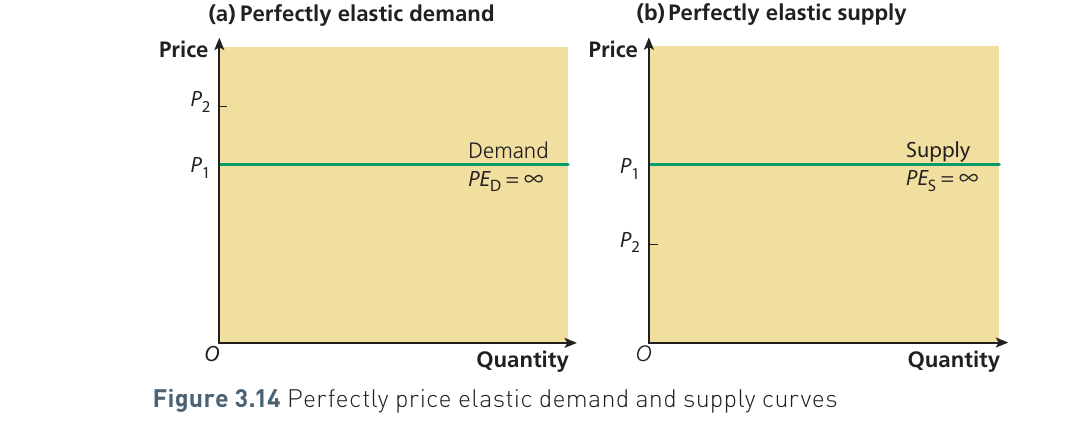
Perfectly elastic demand (PED = ∞)

When demand is infinitely price elastic, the demand curve is horizontal. At prices above the demand curve (for example, above $P_1$), consumers demand zero quantity. At exactly $P_1$, consumers are willing to buy any quantity. Below $P_1$, demand becomes infinite.

This occurs when perfect substitutes are available. If the price rises even slightly above the going rate, consumers immediately switch all their spending to alternative products whose prices have not changed. The quantity demanded immediately falls to zero.

Perfectly elastic supply (PES = ∞)

When supply is infinitely price elastic, the supply curve is horizontal. At prices below the supply curve (for example, below $P_1$), firms supply nothing. At exactly $P_1$, firms are willing to supply any quantity. Above $P_1$, supply becomes infinite.

Although this appears similar to perfectly elastic demand, there is an important difference. $P_1$ represents the minimum price acceptable to firms - the lowest price at which they can cover their costs and remain in the market. If the price falls below $P_1$, firms leave the market entirely because they cannot make sufficient profit. The incentive to stay in the market disappears at any lower price, and firms exit completely.

Remember!