The Travelling Salesperson Problem Revision Notes for AQA A-Level Further Maths

The Travelling Salesperson Problem

Introduction to the problem

A salesperson must visit multiple locations and return to their starting point as efficiently as possible. This situation forms the basis of an important optimization problem in graph theory.

infoNote

The travelling salesman problem is one of the most studied problems in computational mathematics and has practical applications in logistics, manufacturing, DNA sequencing, and circuit board design.

The travelling salesman problem asks you to find a route that visits every vertex of a network and returns to the starting vertex in the shortest possible total distance.

A Hamiltonian cycle (also called a Hamiltonian tour) is a closed path that visits every vertex of a network exactly once before returning to the start.

Classical TSP vs practical TSP

The classical travelling salesman problem requires you to visit every vertex of a network exactly once and return to the start in the minimum possible distance. In other words, you need to find a minimum weight Hamiltonian cycle.

However, real-world situations may not match this classical pattern. Two main issues can arise:

chatImportant

Common Issues with Practical TSP:

No Hamiltonian cycle exists: Some networks cannot be traversed by visiting each vertex exactly once. For instance, any complete tour of certain graphs would require visiting some vertices multiple times.
Triangle inequality not satisfied: The network may violate the triangle inequality, particularly when weights represent travel times. In such cases, the direct route between two vertices might not be the quickest path.

When facing a practical TSP that doesn't fit the classical model, you convert it to an equivalent classical problem first.

Converting practical TSP to classical TSP

To solve a practical TSP with $n$ vertices, follow these steps:

Create a complete network $K_n$ containing the shortest distances between every pair of vertices
Find a minimum weight Hamiltonian cycle for this complete network (this is now a classical problem)
Interpret the solution in the context of the original practical situation

lightbulbExample

Worked Example 1: Converting to a Complete Network

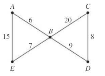
Consider this network where a Hamiltonian cycle exists ( $ABCA$ with total weight 36), but the best practical solution is actually $ACBCA$ with total weight 32.

Solution:

First, construct the complete network $K_5$ by finding shortest distances between all pairs of vertices. For example, the shortest distance from $A$ to $E$ is 13 (using route $ABE$ ) rather than the direct edge weight of 15.

The complete network shows all shortest paths. By inspection, the minimum Hamiltonian tour is $ABDCEA = 60$ .

To interpret this for the original network:

Shortest distance $CE = CDBE = 24$
Shortest distance $EA = EBA = 13$

Therefore, the solution to the practical problem is $ABDCDBEBA = 60$ .

Finding the optimal solution

The only certain way to find the best tour is to check every possible Hamiltonian cycle.

For a complete network $K_n$ with $n$ vertices, there are $(n-1)$ possible first arcs to travel, then $(n-2)$ second arcs, and so on. Since each tour can be listed twice (forwards and backwards), the formula becomes:

chatImportant

A network with $n$ vertices has $\displaystyle\frac{1}{2}(n-1)!$ possible tours.

This number grows exponentially. Even for relatively small networks, checking every cycle becomes computationally impossible. For example, a network with 10 vertices has $\displaystyle\frac{1}{2}(9!) = 181,440$ possible tours.

Because of this exponential growth, you need methods to:

Find a good (though not necessarily optimal) solution within reasonable time
Determine whether your solution is sufficiently close to optimal

Heuristic algorithms

A heuristic algorithm finds a good solution that may not be perfect. For the TSP, a simple heuristic method is the nearest neighbour algorithm, which is an example of a greedy algorithm.

infoNote

Heuristic algorithms trade optimality for speed. While they don't guarantee the best possible solution, they can find very good solutions quickly, making them practical for large-scale problems where finding the exact optimal solution would take too long.

The nearest neighbour algorithm

Step 1: Choose a starting vertex $V$

Step 2: From your current position, choose the arc with minimum weight leading to an unvisited vertex. Travel to that vertex.

Step 3: If unvisited vertices remain, return to Step 2

Step 4: Travel back to $V$

If multiple arcs have equal weight at Step 2, choose one at random. You can rerun the algorithm with different choices to see if they produce better solutions.

infoNote

Important Strategy:

You should repeat the algorithm starting from each vertex in turn. This generates several different tours, from which you select the best.

Note: The 'starting vertex' in the algorithm refers to where you begin the process of finding a tour. Once you have identified a tour, you can start your actual journey at any vertex on that tour.

lightbulbExample

Worked Example 2: Nearest Neighbour Algorithm

This network shows distances (in km) between five towns. Use the nearest neighbour algorithm, starting from each vertex, to find a route for a travelling salesman based at $A$ who must visit every town.

Table

Solution:

Starting from $A$ , the nearest vertex is $C$ (weight $AC = 8$ )

From $C$ , the nearest unvisited vertex is $D$ (weight $CD = 8$ )

From $D$ , the nearest unvisited vertex is $B$ (weight $DB = 10$ )

From $B$ , the nearest unvisited vertex is $E$ (weight $BE = 15$ )

No more unvisited vertices remain, so travel back to $A$ (weight $EA = 14$ )

The total weight for tour $ACDBEA$ is $8 + 8 + 10 + 15 + 14 = 55$

Repeating this process starting from each vertex:

Start vertex	Tour(s)	Total weight
$A$	$ACDBEA$	55
$B$	$BACDEB$	59
$C$	$CABDEC$ , $CDBAEC$	58, 53
$D$	$DCABED$	59
$E$	$ECABDE$ , $ECDBAE$	58, 53

Note that $BACDEB$ and $DCABED$ are the same tour (one is the reverse of the other).

For a salesman based at $A$ , the best tour found is $ABDCEA = 53$ km.

lightbulbExample

Worked Example 3: Practical Application

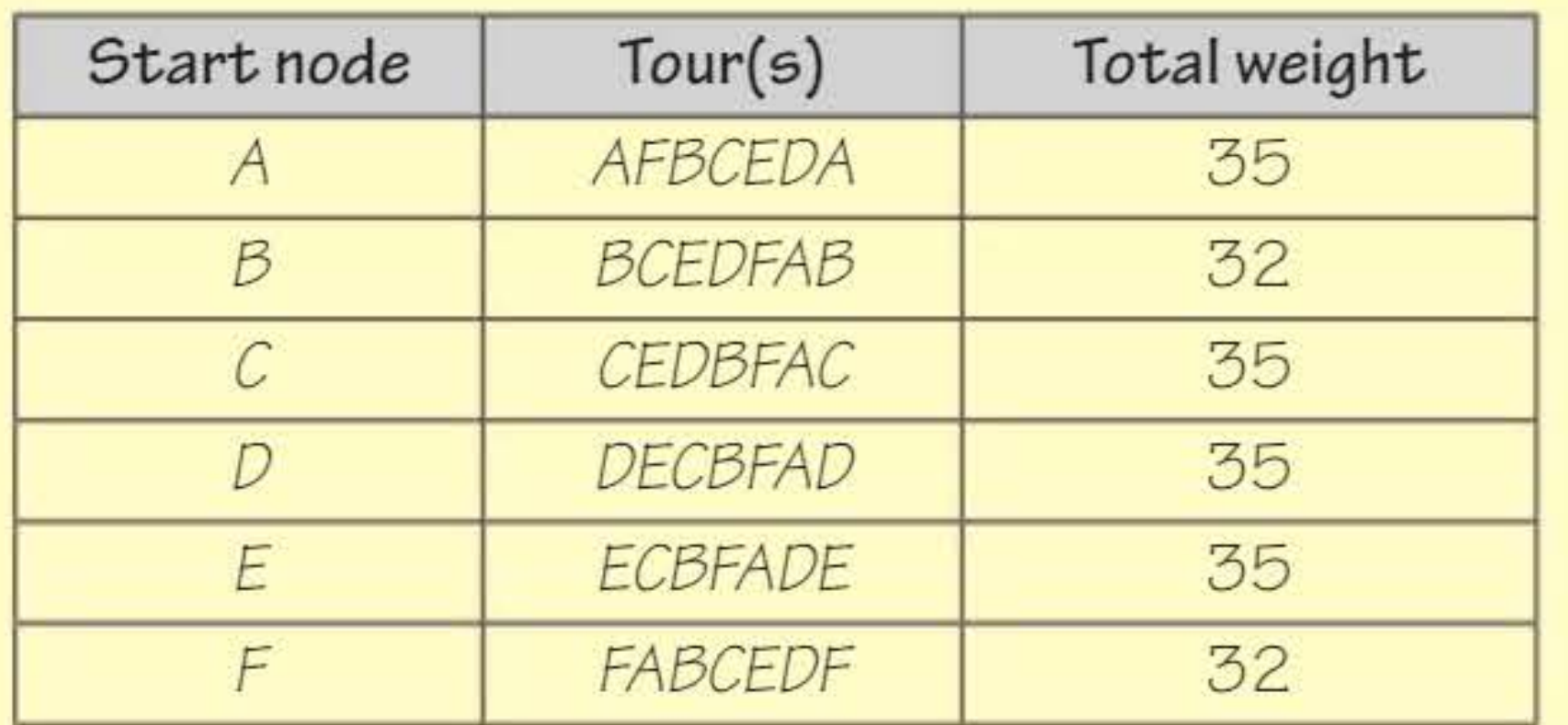
The diagram shows travel times (in minutes) between six locations.

a) Draw a table of shortest travel times.

b) Use the nearest neighbour algorithm to find a solution to the travelling salesman problem. List the route the salesperson will take.

c) Show by inspection that the solution found in b is not optimal.

Solution:

a) The minimum travel times between all pairs of vertices are:

	$A$	$B$	$C$	$D$	$E$	$F$
$A$	-	7	10	15	12	5
$B$	7	-	3	8	5	6
$C$	10	3	-	5	2	9
$D$	15	8	5	-	4	11
$E$	12	5	2	4	-	7
$F$	5	6	9	11	7	-

b) Starting from $A$ , the nearest vertex is $F$ ( $AF = 5$ )

From $F$ , the nearest unvisited vertex is $B$ ( $FB = 6$ )

From $B$ , the nearest unvisited vertex is $C$ ( $BC = 3$ )

From $C$ , the nearest unvisited vertex is $E$ ( $CE = 2$ )

From $E$ , the nearest unvisited vertex is $D$ ( $ED = 4$ )

All vertices visited, so return to $A$ ( $DA = 15$ )

The route is $AFBCEDA$ , with total weight $= 35$ minutes.

Repeating from other starting vertices:

Start vertex	Tour(s)	Total weight
$A$	$AFBCEDA$	35
$B$	$BCEDFAB$	32
$C$	$CEDBFAC$	35
$D$	$DECBFAD$	35
$E$	$ECBFADE$	35
$F$	$FABCEDF$	32

The two 32-minute tours are identical. With $A$ as the starting vertex, these give $ABCEDFA$ .

The salesperson travels $ABCEDFA$ , because the shortest route from $D$ to $F$ goes through $E$ .

c) On the original network, the tour $ABCDEFA = 31$ minutes, so the solution found in b is not optimal.

Finding upper bounds

Since no efficient algorithm guarantees finding the optimal solution length $T$ , you need a way to assess whether a solution is good enough. You do this by finding two values called an upper bound and a lower bound, such that:

chatImportant

lower bound $\leq T \leq$ upper bound

The closer these two bounds are to each other, the more accurately you know the length of the optimal tour. You should try to find the smallest possible upper bound and the largest possible lower bound.

If you have found a tour, it is either optimal or longer than optimal. This means:

infoNote

The length of any known tour is an upper bound.

Using the nearest neighbour algorithm automatically provides an upper bound (though not necessarily a good one).

Upper bound using minimum spanning tree

An alternative method uses a minimum spanning tree for the network. You could visit every vertex by travelling once in each direction along every arc of the minimum spanning tree. Therefore:

chatImportant

$(2 \times \text{length of minimum spanning tree})$ is an upper bound.

This is usually not a good upper bound, but you can improve it using short cuts.

lightbulbExample

Worked Example 4: MST and Short Cuts for Upper Bound

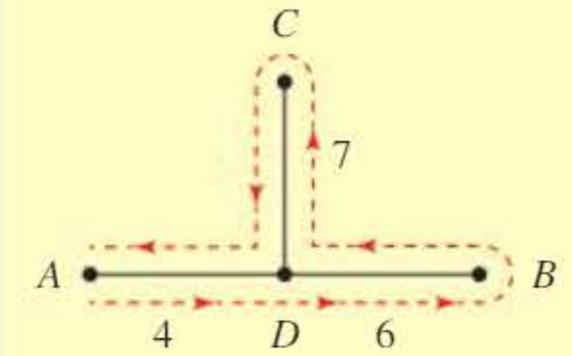
Use the minimum spanning tree (MST) and short cuts to find an upper bound for the optimal solution of the TSP for this network.

Solution:

Using Kruskal's or Prim's algorithm to find two MSTs, each with total length 17:

First MST gives an upper bound of $2 \times 17 = 34$

For the first MST, this upper bound is equivalent to the route $ADBDCDA$ .

To improve this, replace $BDC$ (total weight $6 + 7 = 13$ ) with the direct route $BC$ (weight 10).

This reduces the bound by $13 - 10 = 3$ .

The improved upper bound is $34 - 3 = 19$ .

However, this route $ADBCA$ is now a Hamiltonian tour, so there are no more short cuts possible.

For the second MST, the initial upper bound of 34 is equivalent to the route $BADCDAB$ .

To improve this, replace $CDAB$ (total weight $7 + 4 + 6 = 17$ ) with $CB$ (weight 10).

This reduces the bound by $17 - 10 = 7$ .

The improved upper bound is $34 - 7 = 18$ .

This route $BADCB$ is also a Hamiltonian tour with no further short cuts possible.

Of the two values found, the best upper bound is 18.

Remember: You always want the upper bound to be as small as possible.

Finding lower bounds

In addition to an upper bound, you need to find a lower bound.

Suppose you have a network as shown. The optimal tour enters and leaves vertex $A$ along two of the arcs $AB$ , $AC$ , $AD$ , and $AE$ .

You separate these arcs from the rest of the network. The two arcs involved in the tour must have a combined weight of at least $6 + 7 = 13$ (the sum of the two smallest weights from $A$ ).

The remaining three arcs of the tour connect vertices $B$ , $C$ , $D$ , and $E$ , forming a spanning tree for that subgraph.

The minimum spanning tree for this subgraph has weight $5 + 5 + 9 = 19$ , so the three arcs in the tour must have a total weight of at least 19.

Therefore, the complete tour has a total weight of at least $13 + 19 = 32$ .

This provides a lower bound for the tour.

infoNote

To obtain the best possible lower bound, you could repeat this process by removing each vertex in turn. Removing different vertices gives different lower bounds. You want the lower bound to be as large as possible, so select the largest value obtained.

Algorithm for finding a lower bound

Step 1: Choose a vertex $V$

Step 2: Identify the two lowest weights, $p$ and $q$ , of the arcs connected to $V$

Step 3: Remove $V$ and its connecting arcs from the network. Find the total weight, $m$ , of the minimum spanning tree of the remaining subgraph.

Step 4: Calculate lower bound $= p + q + m$

Step 5: If possible, choose another vertex $V$ and return to Step 2

Choose the largest result obtained as the best lower bound.

lightbulbExample

Worked Example 5: Finding Lower Bounds

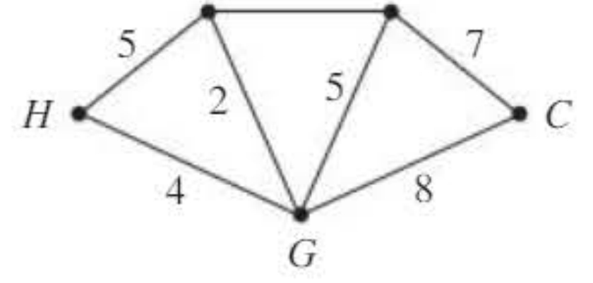
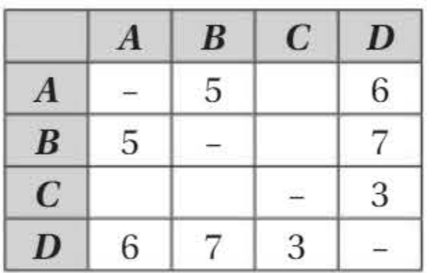
For the network shown:

	$A$	$B$	$C$	$D$	$E$
$A$	-	12	6	7	2
$B$	12	-	9	7	10
$C$	6	9	-	4	8
$D$	7	7	4	-	5
$E$	2	10	8	5	-

a) Find a lower bound for the optimal tour by deleting vertex $A$

b) Find a second lower bound by deleting vertex $B$

c) State which value is the better lower bound

d) Given an upper bound of 32, write an inequality for $T$ , the optimal tour

Solution:

a) The shortest arcs from $A$ are $AC = 6$ and $AE = 2$

Table

The minimum spanning tree is $BD = 7$ , $CD = 4$ , and $DE = 5$ .

Using Prim's algorithm: lower bound $= (6 + 2) + (7 + 4 + 5) = 24$

b) The shortest arcs from $B$ are $BC = 9$ and $BD = 7$

The minimum spanning tree of the remaining vertices is $AE = 2$ , $CD = 4$ , and $DE = 5$ .

Lower bound $= (9 + 7) + (2 + 4 + 5) = 27$

c) Since $27 > 24$ , the better lower bound is 27

d) The optimal tour length $T$ lies between the lower and upper bounds, so $27 \leq T \leq 32$

Note: The arcs forming the better lower bound ( $BC$ , $BD$ , $AE$ , $CD$ , and $DE$ ) do not form a tour themselves. If they did form a tour, you would know that $T = 27$ exactly.

chatImportant

Key Point About Lower Bounds:

If you find a lower bound which forms a tour, then that tour is the optimal solution. If none of the possible lower bounds form a tour, the optimal tour must be greater than the best lower bound.

Summary

bookmarkSummary

Key Points to Remember:

The travelling salesman problem asks for the shortest route that visits every vertex and returns to the start. The classical version requires visiting each vertex exactly once.
Convert a practical TSP to a classical TSP by creating a complete network $K_n$ of shortest distances, then finding a minimum weight Hamiltonian cycle.
There are $\displaystyle\frac{1}{2}(n-1)!$ possible tours in a network with $n$ vertices, making exhaustive checking impractical for large networks.
The nearest neighbour algorithm is a heuristic method that builds a tour by repeatedly choosing the shortest available arc to an unvisited vertex. Run it from each vertex and select the best result.
Upper bounds can be found from any known tour, or by using $(2 \times \text{MST length})$ and applying short cuts to improve it. You want the smallest possible upper bound.
Lower bounds are found by deleting a vertex, taking the sum of its two smallest arcs, and adding the MST of the remaining vertices. Repeat for each vertex and choose the largest result.
The optimal tour length $T$ satisfies: lower bound $\leq T \leq$ upper bound. If a lower bound forms a tour, it is the optimal solution.

The Travelling Salesperson Problem (AQA A-Level Further Maths): Revision Notes