Using the Chi-Squared Test (OCR A-Level Biology A): Revision Notes
Using the Chi-Squared Test
What is the chi-squared test?
The chi-squared test (χ²) is a statistical method used to analyse categorical data — data that can be sorted into distinct groups or categories. This test determines whether differences between what you observe in an experiment and what you expect to happen are likely due to random chance or represent a genuine biological effect.
Chi-squared testing is applicable only to categorical data (data that falls into distinct groups), not continuous numerical measurements. Examples of categorical data include: eye colour (blue, brown, green), wing type (long, vestigial), or blood group (A, B, AB, O).
In genetics, the chi-squared test helps confirm whether experimental crosses produce offspring ratios that match predicted Mendelian ratios. It is particularly useful for testing whether two genes are linked on the same chromosome or assort independently during meiosis.
The null hypothesis
Before conducting a chi-squared test, you must formulate a null hypothesis. This is a statement about the biological system you are investigating that allows you to predict the expected numbers in each category.
For example, in a genetics experiment, your null hypothesis might state: "The two genes are located on different chromosomes and will show independent assortment, producing offspring in a 9:3:3:1 ratio."
The null hypothesis always assumes there is no significant difference between observed and expected results. It typically proposes that any variations are due to random chance, or in genetics, that genes are not linked and follow standard Mendelian inheritance patterns.
The chi-squared test then determines whether your experimental results differ significantly from what this hypothesis predicts. If the difference is small, you accept the null hypothesis. If the difference is large, you reject it and conclude that another factor (such as gene linkage) is affecting the results.
Observed and expected data
Observed data (O) are the actual results you collect during your experiment. These are the real counts or measurements from your practical work.
Expected data (E) are the predicted values based on your null hypothesis. In genetic crosses, these come from theoretical ratios such as:
- 3:1 for a monohybrid cross
- 9:3:3:1 for a dihybrid cross with unlinked genes
- 1:1:1:1 for a dihybrid test cross with unlinked genes
To calculate expected values, multiply the total number of observations by the proportion predicted for each category. For example, if you have offspring and expect a 1:1:1:1 ratio across four categories, each expected value is .
Calculating Expected Values
If you cross two heterozygous organisms and obtain 480 offspring, and your null hypothesis predicts a 3:1 ratio:
- Total offspring = 480
- Expected for dominant phenotype:
- Expected for recessive phenotype:
Always check your expected values sum to the total number of observations!
The chi-squared formula
The chi-squared value is calculated using this formula:
Where:
- means "sum of" — you calculate the value for each category and add them together
- is the observed value for a category
- is the expected value for that category
This formula measures how far each observed value deviates from its expected value, squares these deviations (so positive and negative differences don't cancel out), divides by the expected value (to standardise the differences), and then sums all these values together.
The larger the χ² value, the greater the difference between your observed and expected results.
Calculating degrees of freedom
Degrees of freedom (df) represent the number of categories that can vary independently in your data. This value determines which row of the critical values table you use.
Calculate degrees of freedom using:
Where is the number of categories in your experiment.
For example, if you have four phenotypic categories in a genetic cross (such as four different combinations of traits), your degrees of freedom equals .
Critical values and probability
After calculating your χ² value, compare it to a critical value from a statistical table. Biologists conventionally use the 5% significance level, which corresponds to a probability () of .
This probability represents the chance that the differences between observed and expected values occurred purely by random chance. At , there is a 5% (or 1 in 20) probability that random variation alone could produce the observed results.
Standard Significance Level
The (5%) level is the standard in biology. This means we accept a 5% chance of incorrectly rejecting the null hypothesis. In other words, we're 95% confident in our conclusion when we reject the null hypothesis.
For example, with 3 degrees of freedom at , the critical value is .
Interpreting chi-squared results
Compare your calculated χ² value to the critical value:
If calculated χ² < critical value:
- The difference between observed and expected results is not statistically significant
- The differences are likely due to random chance
- You accept the null hypothesis
- Example: If your calculated χ² is and the critical value is , the probability of getting this result by chance is greater than 5%, so you accept the null hypothesis
If calculated χ² > critical value:
- The difference is statistically significant
- The differences are unlikely to be due to chance alone
- You reject the null hypothesis
- A biological factor (such as gene linkage) is affecting the results
- Example: If your calculated χ² is and the critical value is , the probability of getting this result by chance is less than 5%, so you reject the null hypothesis
Remember the Rule:
- χ² less than critical value → accept null hypothesis → differences due to chance
- χ² greater than critical value → reject null hypothesis → significant difference exists
This is the opposite of what might seem intuitive! A smaller χ² value means your results match expectations better.
Application to genetics: Worked example
Worked Example: Testing for Independent Assortment in Drosophila
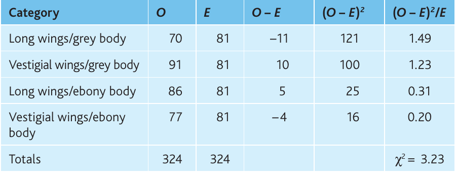
A student performed a test cross between fruit flies (Drosophila melanogaster) showing two traits: wing length (long or vestigial) and body colour (grey or ebony). The expected ratio for a dihybrid test cross with unlinked genes is 1:1:1:1.
Null hypothesis: The genes for wing length and body colour are on different chromosomes and show independent assortment, producing offspring in a 1:1:1:1 ratio.
Here are the results:
Step-by-step calculation:
-
Total offspring:
-
Expected value for each category:
-
Calculate for each category
-
Calculate for each category
-
Calculate for each category
-
Sum all values:
-
Degrees of freedom:
-
Critical value at with 3 df:
Interpretation: The calculated χ² value () is less than the critical value (). This indicates that the probability of obtaining these results by chance is greater than 5%. The difference between observed and expected values is not statistically significant.
Conclusion: Accept the null hypothesis. The two genes are located on different chromosomes and show independent assortment. The small deviations from the expected 1:1:1:1 ratio are likely due to random sampling variation.
Chi-squared and genetic linkage
Chi-squared tests help determine whether genes are linked (on the same chromosome) or show independent assortment (on different chromosomes).
When two genes are on different chromosomes, they assort independently during meiosis. In metaphase I, homologous chromosome pairs can align in two equally probable orientations. This produces four types of gametes in equal proportions ( or each). Random fertilisation then produces the characteristic Mendelian ratios.
Expected Ratios for Independent Assortment
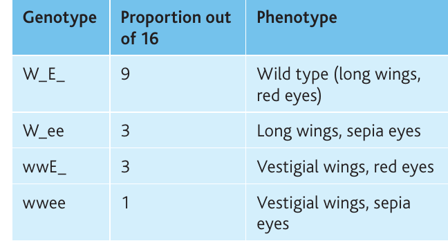
- Dihybrid cross (): Expected phenotypic ratio is 9:3:3:1
- Test cross ( homozygous recessive): Expected ratio is 1:1:1:1
These ratios only occur when genes are on different chromosomes. Significant deviations suggest the genes may be linked.
Example with independent assortment
Students crossed pure-breeding wild-type flies (long wings, red eyes) with flies having vestigial wings and sepia eyes. All offspring showed the wild-type phenotype. The flies were then crossed together, producing these offspring:
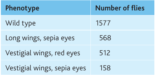
Performing a chi-squared test on these data:
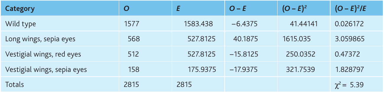
The calculated χ² is with 3 degrees of freedom. The critical value at is . Since , the null hypothesis is accepted. The genes for wing length and eye colour are on different chromosomes and show independent assortment.
Example with gene linkage
When the same students tested wing length alongside a different eye colour gene (cinnabar), they found very different results. In a test cross, they obtained:
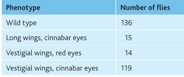
The expected ratio for unlinked genes would be 1:1:1:1 (approximately flies in each category). However, the observed results show two large classes ( and ) and two very small classes ( and ).
Worked Example: Detecting Gene Linkage
A chi-squared test on these data gives χ² = with 3 degrees of freedom. Since , this difference is highly significant (). The null hypothesis is rejected.
Conclusion: The genes for wing length and cinnabar eye colour do not show independent assortment. They are linked on the same chromosome (both are actually on chromosome 2 in Drosophila). This is an example of autosomal linkage.
The two larger classes ( and ) represent parental combinations — these are the original combinations of alleles present in the heterozygous parent. The two smaller classes ( and ) represent recombinant phenotypes produced by crossing over during prophase I of meiosis.
When genes are linked, you typically observe:
- Two large phenotypic classes (parental types) — these maintain the original allele combinations
- Two small phenotypic classes (recombinant types) — these result from crossing over
The closer together two genes are on a chromosome, the less likely crossing over will occur between them, and the smaller the recombinant classes will be.
Remember!
Key Points to Remember:
- The chi-squared test compares observed experimental results with expected values based on a null hypothesis
- Calculate χ² using the formula:
- Degrees of freedom = (where is the number of categories)
- Compare your calculated χ² to the critical value at
- If χ² < critical value: accept the null hypothesis (differences due to chance)
- If χ² > critical value: reject the null hypothesis (differences are significant)
- In genetics, chi-squared tests whether genes are linked or show independent assortment
- Significant deviations from expected Mendelian ratios often indicate gene linkage on the same chromosome