Harder Graphs (Edexcel GCSE Maths): Revision Notes
Harder graphs
Understanding more complex graph types is essential for GCSE mathematics. These graphs go beyond simple linear and quadratic functions to include cubic, exponential, reciprocal, circular, and trigonometric functions. Each type has distinct characteristics that make them recognisable and predictable.
Cubic graphs (x³ graphs)
Cubic graphs follow the general form , where the coefficients b, c, and d can be zero, but the x³ term must be present as the highest power. These graphs are characterised by their distinctive curved shape that includes what mathematicians call a "wiggle" in the middle section.
The direction of a cubic graph depends on the sign of the coefficient of x³. When the coefficient is positive (+x³), the graph rises from bottom left to top right. When the coefficient is negative (-x³), the graph falls from top left to bottom right. This directional behaviour is consistent regardless of the other terms in the equation.
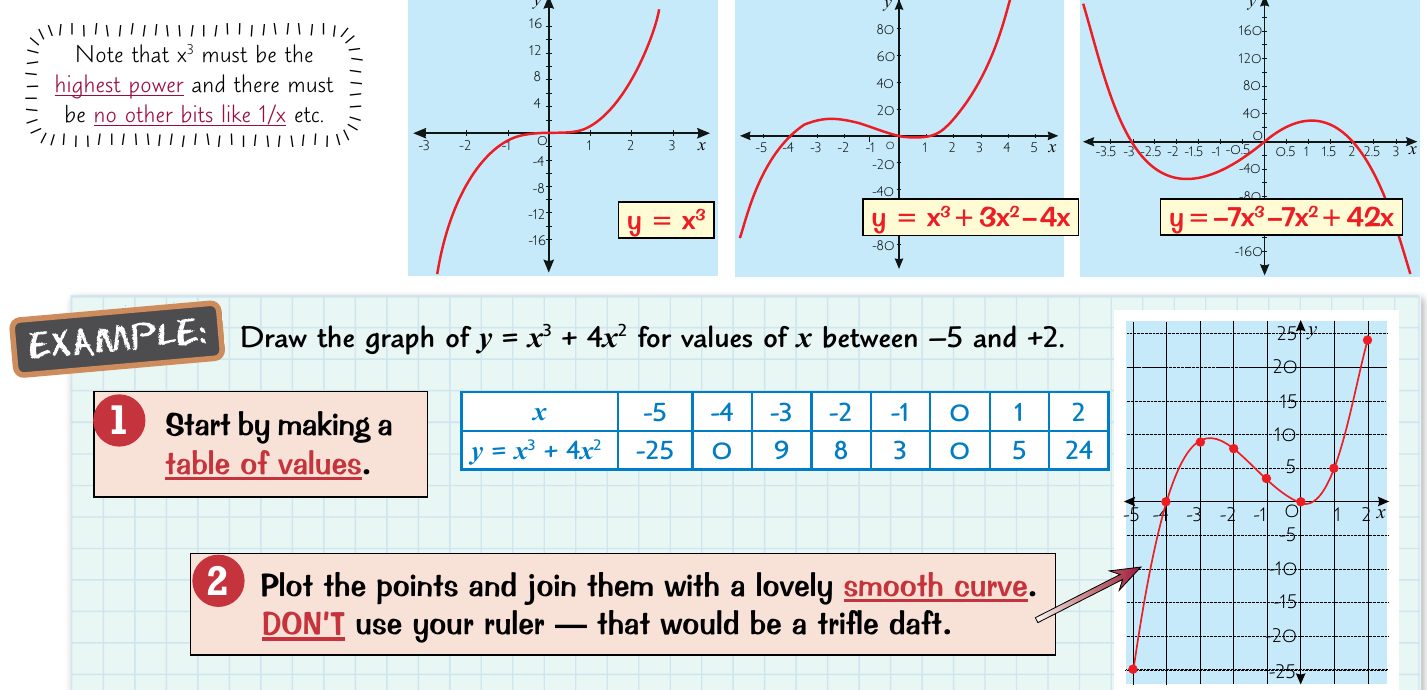
To plot a cubic graph successfully, you should create a table of values by substituting different x-values into the equation. Once you have calculated the corresponding y-values, plot these coordinate points on a grid. The crucial step is connecting these points with a smooth, flowing curve rather than using straight lines between points.
Exponential graphs (k^x graphs)
Exponential graphs have the form where k represents a positive number. These graphs display remarkable consistency in their behaviour, always remaining above the x-axis and passing through the point (0,1) regardless of the value of k.
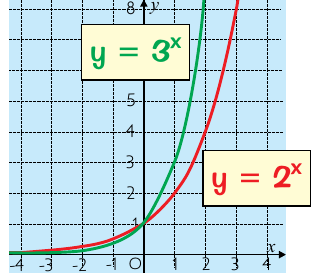
When k is greater than 1 and the power is positive, the graph demonstrates exponential growth, curving upwards dramatically as x increases. The larger the base value k, the more rapid this growth becomes.
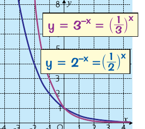
Exponential decay occurs when the power is negative, creating graphs of the form . These graphs still pass through (0,1) but decrease rapidly as x increases, approaching the x-axis but never quite reaching it.
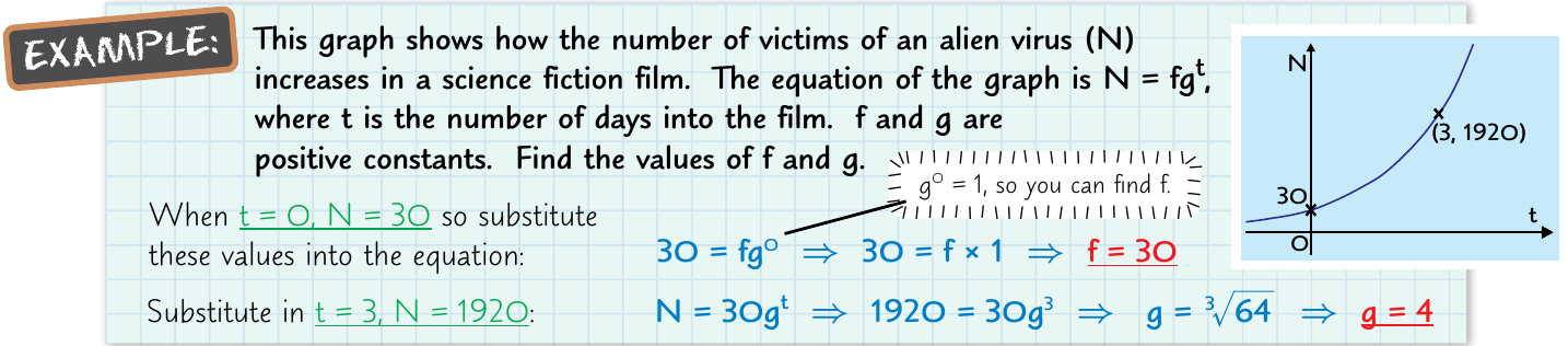
Real-world applications of exponential graphs include population growth, radioactive decay, and compound interest calculations. The alien virus example demonstrates how exponential growth can be modelled mathematically, showing how a small initial population can grow to enormous numbers in a relatively short time.
Reciprocal graphs (1/x graphs)
Reciprocal graphs follow the form or , where A is a constant. These graphs create a distinctive hyperbola shape consisting of two separate branches that never touch each other or the coordinate axes.
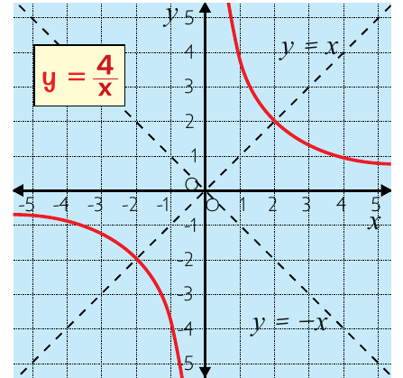
The two branches of a reciprocal graph appear in opposite quadrants - typically the first quadrant (top right) and third quadrant (bottom left) for positive values of A, or the second and fourth quadrants for negative values. These graphs are symmetrical about the lines y = x and y = -x.
An important characteristic of reciprocal graphs is that they have asymptotes - invisible lines that the graph approaches but never crosses. The x-axis and y-axis serve as asymptotes for these functions, which explains why the graph never touches these lines and why the function is undefined when x = 0.
Circle graphs
Circle graphs follow the standard equation , where r represents the radius of the circle. This form assumes the circle is centred at the origin (0,0).
For a circle with centre (0,0) and radius r, you can determine the radius by taking the square root of the constant term in the equation.
Worked Example: Finding the Radius
If , then , so the radius .
When the equation is , the circle has its centre at (0,0) with radius , since the square root of 100 is 10.
Trigonometric graphs
Trigonometric graphs represent periodic functions that repeat their patterns at regular intervals. The two fundamental trigonometric functions you need to understand are sine and cosine.
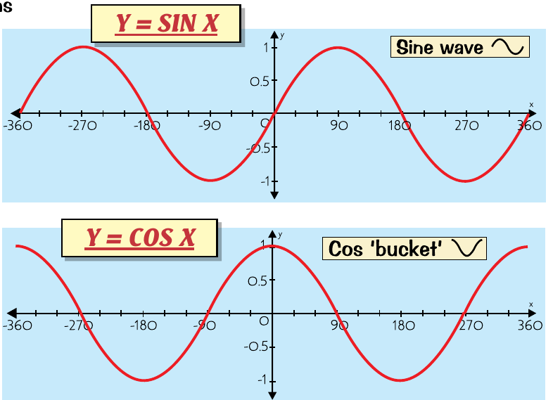
The sine function () creates what's commonly called a "sine wave" - a smooth, rolling curve that oscillates between -1 and +1. The sine graph starts at zero when x = 0 and follows a predictable wave pattern.
The cosine function () produces a "cosine bucket" shape - similar to the sine wave but shifted. The cosine graph starts at its maximum value of 1 when x = 0, creating a pattern that resembles an upside-down bucket.
Both sine and cosine graphs have identical underlying shapes, but the cosine graph is shifted 90 degrees to the right compared to the sine graph. They both oscillate between y-limits of exactly +1 and -1, and both repeat their patterns every 360 degrees.
When drawing extended trigonometric graphs, start by sketching one complete cycle from 0° to 360°, then repeat this pattern in both directions. The key is recognising that these functions are periodic, meaning they repeat their behaviour infinitely in both directions.
General graphing techniques
Regardless of the graph type, certain techniques will help you create accurate representations. Always start by creating a table of values, choosing x-values that will reveal the graph's key features. Plot these points carefully on coordinate axes, then connect them with the appropriate type of curve.
Remember that different graph types require different approaches to curve drawing. Cubic graphs need smooth, flowing curves that capture the wiggle characteristic. Exponential graphs require curves that show rapid change in one direction while approaching an asymptote in the other. Reciprocal graphs need two separate branches that never touch the axes.
Key Points to Remember:
- Cubic graphs () always have a characteristic wiggle and the direction depends on whether the coefficient is positive or negative
- Exponential graphs () always pass through (0,1) and stay above the x-axis
- Reciprocal graphs () form hyperbolas with two branches that never touch the coordinate axes
- Circle graphs follow with the radius found by taking the square root of the constant term
- Trigonometric graphs repeat their patterns: sine waves start at zero, cosine buckets start at maximum value