Graphs of Vertical Projectile Motion Revision Notes for Grade 12 NSC Matric Physical Sciences

Graphs of Vertical Projectile Motion

Understanding vertical projectile motion through graphs is essential for analysing motion under gravity. You can describe any vertical projectile motion using three key graphs: position versus time, velocity versus time, and acceleration versus time. These graphs work together to give you a complete picture of how an object moves when only gravity acts on it.

Understanding graph relationships

Before diving into vertical projectile motion, you need to understand how kinematics graphs relate to each other. The slope and area under the curve of each graph tell you important information about motion.

chatImportant

Fundamental Graph Relationships:

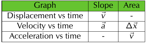
Remember these critical connections between graphs:

The slope of a displacement-time graph gives you velocity
The slope of a velocity-time graph gives you acceleration
The area under a velocity-time graph gives you the change in displacement
The area under an acceleration-time graph gives you the change in velocity

Comparing different types of motion

To understand vertical projectile motion graphs better, let's first compare them with simpler types of motion:

infoNote

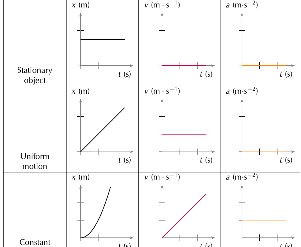
Notice how constant acceleration motion (bottom row) produces three distinct graph shapes:

A curved (parabolic) position-time graph
A straight line velocity-time graph
A horizontal line acceleration-time graph

This is exactly what you see in vertical projectile motion, since gravity provides constant acceleration.

The three cases of vertical projectile motion

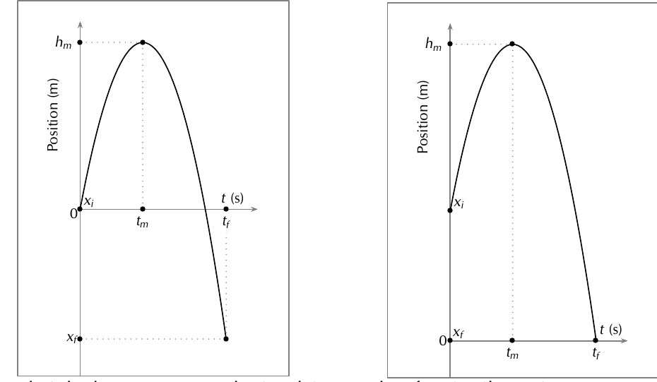
Case 1: object thrown upwards with initial velocity

Position-time graph:

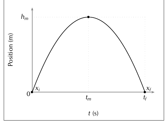
The position graph is parabolic (curved like an upside-down U). The object starts at initial position $x_i$ , rises to maximum height $h_m$ at time $t_m$ , then falls back down to final position $x_f$ at time $t_f$ .

Velocity-time graph:

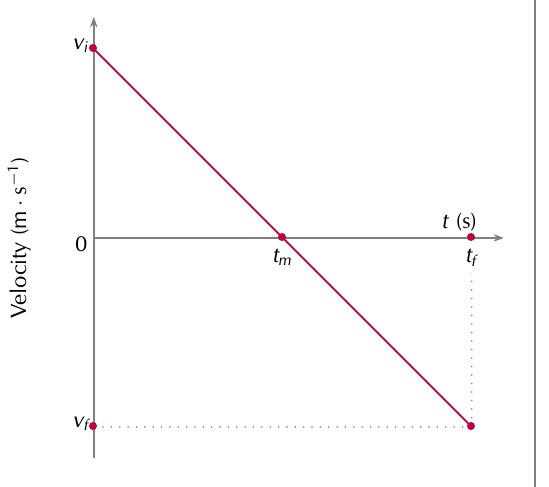
The velocity graph is a straight line with negative slope. The object starts with positive initial velocity $v_i$ (upwards), decreases linearly, reaches zero velocity at maximum height (time $t_m$ ), then continues to negative final velocity $v_f$ (downwards).

Acceleration-time graph:

The acceleration graph shows constant negative acceleration throughout the motion. This represents gravity pulling the object downwards at $-9.8 \,\mathrm{m\,s^{-2}}$ .

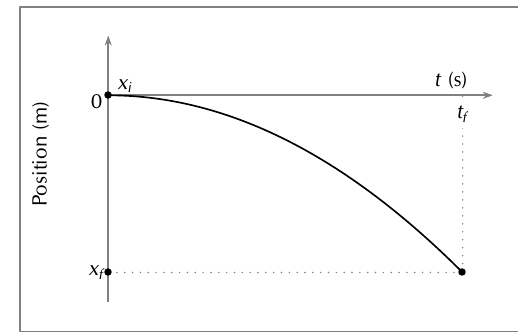
Case 2: object dropped from rest

Position-time graph:

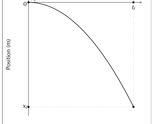
The position starts at zero and curves downward, showing the object falling from rest under gravity's influence.

Velocity-time graph:

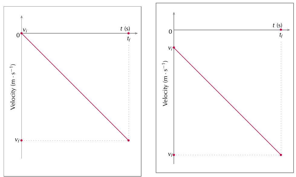
The velocity starts at zero and increases linearly in the negative direction (gaining speed as it falls).

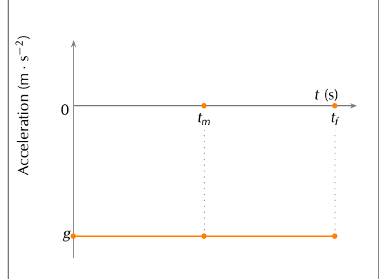
Acceleration-time graph:

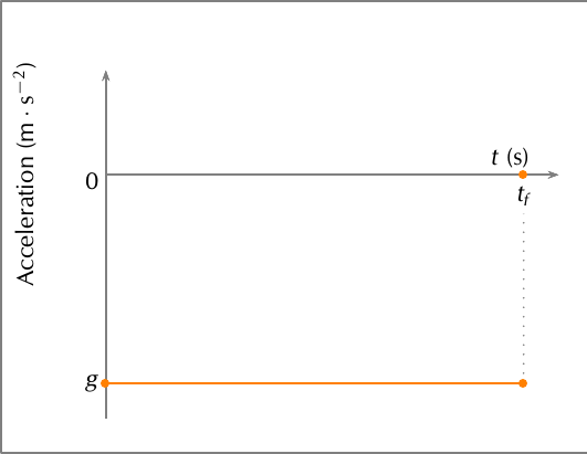
The acceleration remains constant at $-g$ throughout the motion, just like in Case 1.

Case 3: object with initial downward velocity

Position-time graph:

The position curve is steeper than the "dropped from rest" case because the object starts with downward velocity.

chatImportant

Important note about coordinate systems:

The shape and position of your graphs depend on where you choose your origin (reference point). If you place the origin at ground level, a ball thrown from a building will start above zero on the position axis. If you place the origin at the throwing point, it starts at zero.

Key characteristics to remember

Position graphs are always parabolic for constant acceleration motion
Velocity graphs are always straight lines for constant acceleration motion
Acceleration graphs are always horizontal lines for constant acceleration motion
At maximum height, velocity equals zero
The slope of velocity-time graphs always equals $-g$ ( $-9.8 \,\mathrm{m\,s^{-2}}$ )
Upward motion has positive velocity, downward motion has negative velocity (when upward is chosen as positive)

lightbulbExample

Worked Example: Drawing Projectile Motion Graphs

Problem: Stanley tosses a rubber ball upwards from a balcony 20 m above the ground with initial velocity of 4.9 m·s $^{-1}$ . Draw position, velocity, and acceleration graphs.

Solution approach:

Step 1: Calculate the upward motion

Initial velocity: $v_i = +4.9 \,\mathrm{m\,s^{-1}}$
Final velocity at max height: $v_f = 0 \,\mathrm{m\,s^{-1}}$
Acceleration: $g = -9.8 \,\mathrm{m\,s^{-2}}$

Using $v_f^2 = v_i^2 + 2g\Delta x$ :

0^2 = (4.9)^2 + 2(-9.8)\Delta x

\Delta x = +1.225 \,\mathrm{m} \quad \text{(maximum height above balcony)}

Using $v_f = v_i + g t$ :

0 = 4.9 + (-9.8)t

t = 0.5 \,\mathrm{s} \quad \text{(time to reach maximum height)}

Step 2: Calculate the downward motion
Total displacement from maximum height to ground:

\Delta x = -(20 + 1.225) = -21.225 \,\mathrm{m}

Using $\Delta x = v_i t + \tfrac{1}{2} g t^2$ :

-21.225 = 0 + \tfrac{1}{2}(-9.8)t^2

t = 2.08 \,\mathrm{s} \quad \text{(time to fall from maximum height to ground)}

Step 3: Draw the position-time graph
The ball starts at 20 m, rises to 21.225 m at t = 0.5 s, then falls to 0 m at t = 2.58 s total.

Step 4: Draw the velocity-time graph
The velocity starts at +4.9 m·s $^{-1}$ , decreases linearly to 0 at t = 0.5 s, then continues to -20.4 m·s $^{-1}$ at t = 2.58 s.

Step 5: Draw the acceleration-time graph
The acceleration remains constant at -9.8 m·s $^{-2}$ throughout the entire motion.

Analysing projectile motion graphs

From position-time graphs:

Initial position (y-intercept)
Maximum height (peak of parabola)
Total flight time (x-intercept where object hits ground)
Time to reach maximum height (x-coordinate of peak)

From velocity-time graphs:

Initial velocity (y-intercept)
Final velocity (final y-value)
Acceleration (slope of line)
Time when velocity equals zero (x-intercept)

From acceleration-time graphs:

Constant value of gravitational acceleration
Confirmation that motion is under constant acceleration

infoNote

Common Exam Tips:

Always establish your coordinate system first — decide which direction is positive
Remember that $g = -9.8 \,\mathrm{m\,s^{-2}}$ when upward is positive
At maximum height, velocity always equals zero
The motion is symmetrical — time up equals time down for objects returning to the same level
Position graphs are parabolic, velocity graphs are linear, acceleration graphs are constant
Use the area under velocity-time graphs to find displacement
Check your graphs make physical sense — does the object move the way you expect?

Summary

bookmarkSummary

Key Points to Remember:

Position-time graphs for vertical projectile motion are always parabolic curves
Velocity-time graphs are always straight lines with slope equal to gravitational acceleration
Acceleration-time graphs are horizontal lines at $-9.8 \,\mathrm{m\,s^{-2}}$ (when upward is positive)
At maximum height, the velocity is always zero
The slope of each graph tells you about the next type of motion (position → velocity → acceleration)

Graphs of Vertical Projectile Motion (Grade 12 NSC Matric Physical Sciences): Revision Notes