Direct Variation Models Revision Notes for HSC SSCE Mathematics Advanced

Direct Variation Models

Understanding direct variation

Direct variation describes a special type of proportional relationship between two quantities. When one quantity increases, the other increases by a proportional amount. Similarly, when one quantity decreases, the other decreases proportionally. This relationship is fundamental in modelling many real-world situations.

A direct variation is a proportional relationship where one quantity directly varies with respect to a change in another quantity. This means that if there is an increase (or decrease) in one quantity, the other quantity will experience a proportionate increase (or decrease).

infoNote

When quantities are directly related, they move in the same direction - both increasing together or both decreasing together. This proportional change is what makes direct variation such a powerful tool for modelling real-world situations.

The general formula

When a quantity $y$ varies directly with a quantity $x$ or a power of $x$ , we can model this relationship using the formula:

$y = kx^n$

Where:

$k$ is the constant of proportionality, where $k \neq 0$
$n$ is the power of the relationship, where $n > 0$
$x$ is the independent variable
$y$ is the dependent variable

This formula allows us to express how the dependent variable changes in response to changes in the independent variable.

chatImportant

The constant of proportionality $k$ must be non-zero ( $k \neq 0$ ), and the power $n$ must be positive ( $n > 0$ ) for a valid direct variation relationship.

Direct linear variation

The simplest form of direct variation is direct linear variation, which takes the form $y = kx$ where $n = 1$ . Unless a different power or function is specified, assume direct variation refers to a linear relationship.

Graphical representation of direct variation

Let's consider a practical example. The distance $D$ (in metres) that a car travels at a constant speed of 20 m/s varies directly with time $T$ (in seconds). The model is $D = 20T$ , where $n = 1$ and $k = 20$ .

When $n = 1$ , the graph is a straight line through the origin, showing that $D$ increases proportionally with $T$ .

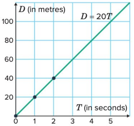
The graph illustrates direct variation, with distance increasing linearly with time. An important characteristic of all direct variation relationships is that they always pass through the origin $(0, 0)$ . This makes sense because when the independent variable is zero, the dependent variable must also be zero.

infoNote

Key Graph Characteristic: All direct variation graphs pass through the origin $(0, 0)$ because when $x = 0$ , we have $y = k(0)^n = 0$ , regardless of the values of $k$ and $n$ .

Finding the constant of proportionality

To apply the direct variation model $y = kx^n$ , we need to determine the constant $k$ using a known pair of values for $x$ and $y$ . Once we have found $k$ , we can use the model to calculate other values.

Simple example

For instance, if $y$ varies directly with $x$ (where $n = 1$ ) and $y = 30$ when $x = 5$ , we can find $k$ as follows:

The model is y = 6x, which can now be used to find $y$ for other values of $x$ .

Worked example 1: Linear variation

lightbulbExample

Worked Example: Machine Hire Cost

The cost $C$ (in dollars) of hiring a machine varies directly with the time $T$ (in days). If $C = 150$ dollars for $T = 3$ days:

Part a: Find the constant of linear proportionality, $k$ .

Strategy: Model the relationship as $C = kT$ and substitute $C = 150$ , $T = 3$ to solve for $k$ .

Solution:

$C = kT$ — Write the direct variation model

$150 = k \times 3$ — Substitute $C = 150$ and $T = 3$

$k = \frac{150}{3}$ — Divide both sides by 3

$k = 50$ — Evaluate

The constant of proportionality is k = 50.

Part b: Find the cost for $T = 7$ days.

Strategy: Use the model $C = 50T$ and substitute $T = 7$ .

Solution:

$C = 50T$ — Write the model with $k = 50$

$C = 50 \times 7$ — Substitute $T = 7$

$C = 350$ — Evaluate

The cost is $350.

Applications of direct variation

Direct variation models help us solve real-world problems where one quantity increases as another increases. This contrasts with inverse variation, where one quantity decreases as another increases. Let's explore applications involving different powers.

Worked example 2: Quadratic variation

lightbulbExample

Worked Example: Area of a Circle

The area $A$ (in square metres) of a circle varies directly with the square of its radius $R$ (in metres). If $A = 12.56$ square metres when $R = 2$ metres:

Part a: Find the constant of proportionality $k$ .

Strategy: Model the relationship as $A = kR^2$ and substitute $A = 12.56$ , $R = 2$ to solve for $k$ .

Solution:

$A = kR^2$ — Write the model with $n = 2$

$12.56 = k \times 2^2$ — Substitute $A = 12.56$ and $R = 2$

$12.56 = k \times 4$ — Evaluate $2^2$

$k = \frac{12.56}{4}$ — Divide both sides by 4

$k = 3.14$ — Evaluate

The constant of proportionality is k = 3.14, approximately $\pi$ .

Part b: Find the radius when $A = 28.26$ square metres, rounded to two decimal places.

Strategy: Use $A = 3.14R^2$ and substitute $A = 28.26$ to solve for $R$ .

Solution:

$A = 3.14R^2$ — Write the model with $k = 3.14$

$28.26 = 3.14R^2$ — Substitute $A = 28.26$

$R^2 = \frac{28.26}{3.14}$ — Divide both sides by 3.14

$R^2 = 9$ — Evaluate

$R = \sqrt{9}$ — Take the positive square root

$R = 3$ — Evaluate

The radius is 3 metres.

Checking our work: Using the exact value $k = \pi$ , the calculation yields $R^2 = \frac{28.26}{\pi} = 9$ , so $R = 3$ metres, confirming the result.

infoNote

When working with quadratic variation ( $n = 2$ ), the relationship involves the square of the independent variable. This is common in geometric formulas involving area, as seen with circles, squares, and other two-dimensional shapes.

Worked example 3: Cubic variation

lightbulbExample

Worked Example: Volume of a Sphere

The volume $V$ (in cubic metres) of a sphere varies directly with the cube of its radius $R$ (in metres). If $V = 36\pi$ cubic metres when $R = 3$ metres:

Part a: Find the constant of proportionality $k$ .

Strategy: Model the relationship as $V = kR^3$ and substitute $V = 36\pi$ , $R = 3$ to solve for $k$ .

Solution:

$V = kR^3$ — Write the model with $n = 3$

$36\pi = k \times 3^3$ — Substitute $V = 36\pi$ and $R = 3$

$36\pi = k \times 27$ — Evaluate $3^3$

$k = \frac{36\pi}{27}$ — Divide both sides by 27

$k = \frac{4\pi}{3}$ — Simplify

The constant of proportionality is k = $\frac{4\pi}{3}$ .

Part b: Find the exact volume when $R = 6$ metres.

Strategy: Use $V = \frac{4\pi}{3}R^3$ and substitute $R = 6$ .

Solution:

$V = \frac{4\pi}{3}R^3$ — Write the model with $k = \frac{4\pi}{3}$

$V = \frac{4\pi}{3} \times 6^3$ — Substitute $R = 6$

$V = \frac{4\pi}{3} \times 216$ — Evaluate $6^3$

$V = 288\pi$ — Simplify

The volume is $288\pi$ cubic metres.

Checking our work: The volume formula for a sphere is $V = \frac{4}{3}\pi R^3$ , which matches our model, confirming the calculations.

chatImportant

Understanding Different Powers:

Linear variation ( $n = 1$ ) represents a constant rate of change
Quadratic variation ( $n = 2$ ) commonly appears in area calculations
Cubic variation ( $n = 3$ ) is found in volume calculations

The power $n$ determines how quickly the dependent variable changes as the independent variable increases.

Remember!

bookmarkSummary

Key Points to Remember:

Direct variation occurs when both quantities increase or decrease together in a proportional relationship, modelled as $y = kx^n$ where $k \neq 0$ is the constant of proportionality and $n > 0$ is the power.
Graphs of direct variation always pass through the origin $(0, 0)$ , because when one variable is zero, the other must also be zero.
To solve problems, first find the constant $k$ by substituting known values into the model, then use the complete model to calculate unknown quantities.
Different powers represent different relationships: $n = 1$ gives linear variation, $n = 2$ gives quadratic variation (like area of circles), and $n = 3$ gives cubic variation (like volume of spheres).
The constant of proportionality $k$ represents the rate at which the dependent variable changes relative to the independent variable raised to the power $n$ .

Direct Variation Models (HSC SSCE Mathematics Advanced): Revision Notes