Linear and Quadratic Rates of Change Revision Notes for HSC SSCE Mathematics Advanced

Linear and Quadratic Rates of Change

Introduction

After studying this topic, you will be able to:

Identify that the rate of change for a linear function is constant and equal to its gradient
Recognise that the rate of change for a non-linear function is variable
Determine the rate of change for linear models in practical contexts
Estimate the instantaneous rate of change for non-linear functions from a graph

infoNote

Understanding rates of change is fundamental to analyzing how quantities vary in real-world situations. Linear relationships show steady change, while non-linear relationships involve varying rates of change.

Constant rate of change in linear models

Understanding linear functions

A linear function is a mathematical relationship where the output changes at a constant rate with respect to the input. The general form of a linear function is $y = mx + c$ , where:

$m$ is the gradient (or slope) of the line
$c$ is the y-intercept (where the line crosses the y-axis)
Both $m$ and $c$ are constants

When we graph a linear function, it always produces a straight line. This straight line tells us that the relationship between the variables doesn't change as we move along the graph.

chatImportant

The defining characteristic of a linear function is its constant rate of change. No matter which two points you choose on a linear graph, the gradient between them will always be the same.

Rate of change in linear functions

For any linear function $y = mx + c$ , the rate of change is constant and equals the gradient $m$ . This means that no matter where we are on the line, the function is changing at the same rate.

$\text{Rate of change} = m$

where $m$ is the gradient of the linear function.

In practical situations, this constant rate represents steady changes such as:

Constant speed (distance changing steadily over time)
Fixed hourly wages (earnings changing steadily with hours worked)
Regular savings (money accumulating at a fixed rate)

Visualising constant rate of change

Let's examine how a constant rate of change appears on a graph:

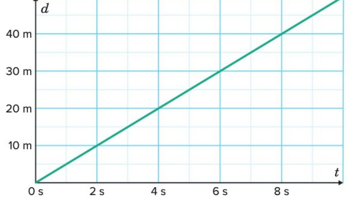
The graph shows $d(t) = 5t$ , where $d$ represents distance in metres and $t$ represents time in seconds. Notice that the line is perfectly straight, indicating that the speed is constant.

infoNote

The straight line has a constant gradient of 5, which means the object is travelling at a constant speed of 5 m·s $^{-1}$ . Whether we measure between 0 and 2 seconds, or between 6 and 8 seconds, the distance changes by exactly 5 metres for every 1 second that passes.

Worked example: Worker earnings

Let's apply our understanding of constant rates of change to a real-world scenario.

lightbulbExample

Worked Example: Worker Earnings

Problem: A worker earns according to the linear model $E(t) = 25t + 50$ , where $E$ is earnings in dollars and $t$ is hours worked. Determine the rate of change and interpret it in context.

Solution:

Step 1: Identify the gradient

We need to identify the gradient $m$ from the linear function $E(t) = 25t + 50$ .

Comparing with the general form $y = mx + c$ , we can see that $m = 25$ .

Step 2: Calculate the rate of change

$\text{Rate of change} = m$

$= 25$

The gradient is the coefficient of $t$ , which we extract from $E(t) = 25t + 50$ .

Step 3: Interpret in context

The rate of change is 25 dollars per hour, meaning the worker earns $25 for each hour worked.

Step 4: Reflect

The constant rate reflects a fixed hourly wage, which is consistent with the linear model. The 50 in the equation represents a fixed payment (perhaps a base payment or allowance) that doesn't change with hours worked.

chatImportant

Key insight: In a linear function $y = mx + c$ , the rate of change is the constant gradient $m$ , representing steady rates in contexts like wages or speed.

Variable rates in quadratic functions

Understanding quadratic functions

Unlike linear functions, quadratic functions produce curved graphs rather than straight lines. A quadratic function has the general form:

$ax^2 + bx + c = 0$

where $a \neq 0$ , and $b$ and $c$ are constants.

The key characteristic of quadratic functions is that their rate of change is not constant. The curve gets steeper or shallower as we move along it, meaning the relationship between variables is accelerating or decelerating.

chatImportant

The fundamental difference between linear and quadratic functions:

Linear functions: Constant rate of change (straight line)
Quadratic functions: Variable rate of change (curved line)

Instantaneous rate of change

For non-linear functions like quadratics, we need a new concept called the instantaneous rate of change. This is:

infoNote

The rate of change at a particular moment in time. For curves, this equals the gradient of the tangent line at a specific point on the graph.

Think of it like checking your speedometer at an exact moment during a car journey where you're accelerating. Your speed is constantly changing, but the speedometer shows your speed at that precise instant.

Visualising variable rates of change

Consider a quadratic distance-time relationship:

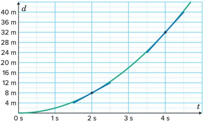
The curve shows $d(t) = 2t^2$ . Notice how the gradient becomes steeper as time increases. The gradient at $x = 4$ is greater than the gradient at $x = 2$ , indicating a higher instantaneous rate of change as time progresses. This represents accelerating motion.

To find the instantaneous rate at any point on a curve, we calculate the gradient of the tangent line at that point. Since we can't always draw perfect tangents, we use a practical method: we estimate the instantaneous rate at a point by calculating the gradient of the secant line connecting $(x, f(x))$ and $(x + h, f(x + h))$ , where $h$ is a small value.

infoNote

A secant line is a straight line that cuts through the curve at two points. When these points are close together, the secant line approximates the tangent line, giving us a good estimate of the instantaneous rate.

Worked example: Tank volume

lightbulbExample

Worked Example: Tank Volume

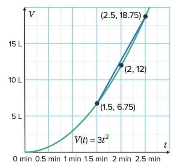
Problem: The volume of water in a tank is modelled by the graph shown, where $V$ is in litres and $t$ is in minutes. Estimate the instantaneous rate of change of volume at $t = 2$ minutes using the secant line.

Solution:

Step 1: Identify the points

We use the graph to identify the points $(1.5, V(1.5))$ and $(2.5, V(2.5))$ on $V(t) = 3t^2$ . These points will define our secant line, which approximates the tangent at $t = 2$ .

From the graph, the points are $(1.5, 6.75)$ and $(2.5, 18.75)$ .

Step 2: Write the formula

$\text{Instantaneous rate} = \frac{d(t_2) - d(t_1)}{t_2 - t_1}$

Step 3: Substitute the values

$= \frac{V(2.5) - V(1.5)}{2.5 - 1.5}$

Step 4: Calculate

$= \frac{18.75 - 6.75}{2.5 - 1.5}$

Substitute $V(2.5) = 18.75$ and $V(1.5) = 6.75$

$= \frac{12}{1}$

$= 12$

Evaluate the expression

Step 5: State the result

The instantaneous rate of change at $t = 2$ is approximately 12 L/min.

Step 6: Reflect

The secant line through $t = 1.5$ and $t = 2.5$ approximates the tangent at $t = 2$ , reflecting the rate at which water is being added to the tank at that specific moment.

chatImportant

Key insight: In quadratic functions, the rate of change varies. The instantaneous rate at a point is the gradient of the tangent, estimated by calculating the gradient of the secant line between $(x, f(x))$ and $(x + h, f(x + h))$ , where $h$ is small.

Remember!

bookmarkSummary

Key Points to Remember:

Linear functions ( $y = mx + c$ ) have a constant rate of change equal to the gradient $m$ . This represents steady rates like constant speed or fixed wages.
Quadratic functions ( $ax^2 + bx + c = 0$ ) have variable rates of change. The curve gets steeper or shallower, representing acceleration or deceleration.
The instantaneous rate of change for a curve is the gradient of the tangent at a specific point. This tells us how fast something is changing at that exact moment.
To estimate the instantaneous rate, calculate the gradient of a secant line connecting two nearby points: $\frac{f(x + h) - f(x)}{h}$ , where $h$ is small.
In exam questions, look for keywords: "constant rate" suggests linear functions, while "instantaneous rate" or "at a particular moment" suggests non-linear functions requiring tangent calculations.

Linear and Quadratic Rates of Change (HSC SSCE Mathematics Advanced): Revision Notes