Linear Models (HSC SSCE Mathematics Advanced): Revision Notes
Linear Models
Introduction to linear models
Linear models are mathematical tools that help us represent and understand real-world situations involving straight-line relationships. These models are extremely useful because many practical scenarios involve quantities that change at a constant rate, such as fuel consumption, costs over time, or water draining from a container.
When we create a linear model, we use equations or inequalities to describe how one quantity changes in relation to another. This allows us to make predictions, solve problems, and understand the relationships between different variables in real situations.
Linear models are particularly powerful for scenarios where:
- Quantities change at a constant rate
- Relationships between variables form straight lines
- Predictions based on consistent patterns are needed
Understanding variables in linear models
In any linear model, we work with two types of variables that represent different aspects of the situation.
Independent variable
The independent variable represents the input values in a relationship. This is the quantity that we can control or that changes independently. In most graphs, this variable is shown on the horizontal axis. For example, if we're modelling fuel consumption over a journey, the distance travelled would be the independent variable because it's what we're measuring along.
Dependent variable
The dependent variable represents the output values that depend on the independent variable. This quantity changes in response to changes in the independent variable. On a graph, the dependent variable appears on the vertical axis. Continuing our fuel example, the volume of fuel remaining would be the dependent variable because it depends on how far we've travelled.
In real-world contexts, these variables often represent physical quantities like time, distance, cost, mass, volume, or temperature. Choosing appropriate variables with correct units of measurement is crucial for creating an accurate model.
Gradient and vertical intercept in context
When working with linear models, two key features help us understand the situation: the gradient and the vertical intercept. Let's explore what these mean in practical contexts.
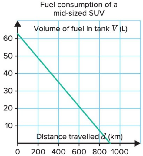
Consider the example of modelling fuel consumption in a car. Instead of using generic variables like and , we can choose variables that better represent the context:
- The independent variable might represent distance travelled, measured in kilometres (we could use for distance)
- The dependent variable might represent volume of fuel remaining, measured in litres (we could use for volume)
This makes the model more meaningful and easier to interpret.
The vertical intercept as an initial value
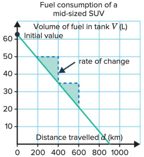
In linear modelling situations, the vertical intercept is often called the initial value because it represents the starting point before any change has occurred. Looking at the fuel consumption graph, the vertical intercept is litres. This represents the volume of fuel in a full tank before the car begins its journey.
The gradient as a rate of change
The gradient in a linear model represents a rate of change. This tells us how quickly one quantity changes relative to another. In the fuel consumption example, the gradient measures the car's fuel consumption rate, expressed in litres per kilometre (L/km) or litres per 100 kilometres (L/100 km).
The rate of change describes how the function's value changes as the independent variable changes. For instance, a gradient of in our fuel example would mean the car uses litres for every kilometre travelled, or litres per kilometres.
Important considerations for context
Linear graphs can theoretically extend indefinitely in both directions. However, many physical quantities cannot be negative.
When working with a linear model, always consider which values make sense in the given context:
- Distance, volume, and time cannot have negative values in most real situations
- Linear models often exist primarily in the first quadrant of the coordinate plane
- Temperature is an exception where negative values are meaningful
Worked example 1: Water draining from a bucket
Worked Example: Water Draining from a Bucket
A bucket initially full of water has a hole in its side. The graph shows the amount of water remaining over time.
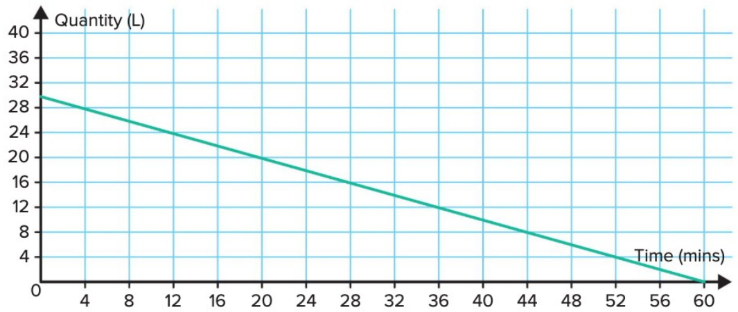
Part a: Determine the gradient of the function
To find the gradient, we use the formula:
From the graph, we can identify two clear points: and .
The rise is units down, which we write as .
The run is units across.
Part b: Determine the vertical intercept
Looking at where the line crosses the vertical axis, we can see this occurs at . Therefore, the vertical intercept is 30.
Part c: Explain what the gradient represents in this context
The gradient represents the rate of change between the two physical quantities being measured. In this situation, it shows how the amount of water in the bucket changes over time.
A gradient of means the amount of water in the bucket decreases by 1 litre every 2 minutes. In other words, litre of water drains out through the hole every minutes.
Part d: Explain what the vertical intercept represents in this context
The vertical intercept represents the initial value - the starting amount before any change occurs. In this case, the vertical intercept of represents the initial amount of water in the bucket before water began draining out through the hole. The bucket initially contained 30 litres.
Part e: Determine an equation using appropriate variables
To create an equation for this situation, we should choose variables that represent the context clearly. Let's use:
- for volume (the dependent variable, measured in litres)
- for time (the independent variable, measured in minutes)
Starting with the general form , we substitute our variables:
Here, (the gradient) and (the vertical intercept).
The equation describes the volume of water remaining in the bucket after minutes.
Part f: Determine the amount of water remaining after 20 minutes
To find this, we substitute into our equation:
After minutes, there are 20 litres of water remaining in the bucket.
Worked example 2: Burning candle
Worked Example: Burning Candle
A candle with height cm burns according to the equation , where is the time elapsed in minutes.
Part a: Complete the table of values
| Time ( min) | 0 | 1 | 2 | 3 |
|---|---|---|---|---|
| Height of candle ( cm) | 8 | 6 | 4 | 2 |
To complete this table, we substitute each value of into the equation:
When :
When :
When :
When :
Part b: Sketch the graph
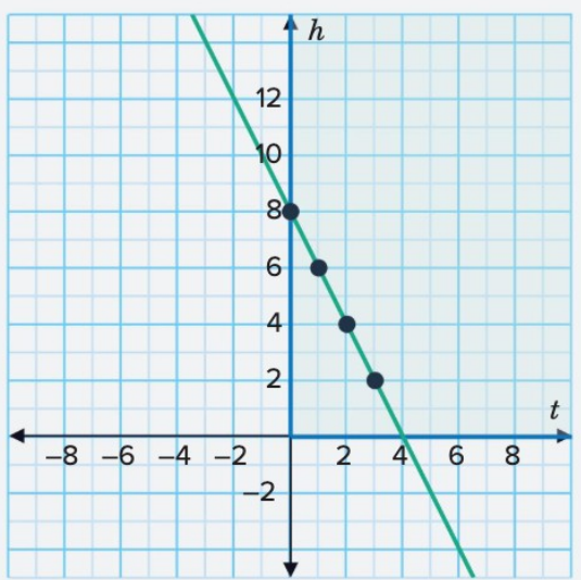
To sketch the graph, we plot the points from our table: , , , and . Then we draw a straight line through these points.
Part c: Determine the valid domain for the model
Physical constraints affect which values make sense in this model. Both the height of a candle and elapsed time cannot be negative values in reality. Therefore, we need and .
Looking at the graph in the first quadrant, we can see the model is only valid when 0 ≤ t ≤ 4. When , the equation gives , meaning the candle has completely burned down. The equation accurately models the candle's height in the first quadrant only.
Worked example 3: Carpenter's charges
Worked Example: Carpenter's Charges
A carpenter charges a call-out fee of $150 plus $45 per hour for work.
Part a: Determine an equation for the total amount charged
We need to express the relationship:
Total amount charged = $45 × Number of hours + $150
Using appropriate variables:
- Let represent the total cost (dependent variable)
- Let represent the number of hours worked (independent variable)
Starting with the general form and substituting:
Here, (the gradient, representing the hourly rate) and (the vertical intercept, representing the call-out fee).
Part b: Determine the total amount charged for 6 hours of work
We substitute into the equation:
The total amount charged is $420.
Part c: Determine the number of hours worked if the total charge is $735
This time we know the cost and need to find the hours. We substitute and solve for :
The carpenter worked for 13 hours.
Modelling with linear inequalities
Linear inequalities are used to model situations involving constraints or limits. Many real-world problems involve maximum or minimum values, budgets, or capacity restrictions. While the inequality can be solved mathematically, the solution must be interpreted carefully in context.
A viable solution satisfies the inequality and makes practical sense in the situation. For example, if we're counting items, whole numbers are viable.
A non-viable solution might satisfy the inequality mathematically but isn't realistic in the real-world context. For example, negative items or fractional items when only whole items are possible.
Steps for modelling with inequalities
When modelling real-world situations using linear inequalities:
- Define a variable (e.g., for number of items) and write an inequality based on the problem's constraints
- Solve the inequality algebraically to find the solution set
- Interpret the solution in context, identifying viable solutions (e.g., whole numbers for items) and non-viable solutions (e.g., negative quantities)
- Graph the solution on a number line, highlighting viable solutions
Important rule for inequalities
When multiplying or dividing both sides of an inequality by a negative number, the inequality sign must be reversed to maintain the truth of the statement. This is a crucial rule that students often forget.
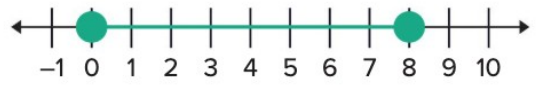
For example, if modelling a budget inequality (where represents items costing $5 each), the solution is graphed on a number line. Viable solutions are whole numbers from to , as items cannot be negative or fractional.
Worked example 4: Hairstyling cost
Worked Example: Hairstyling Cost
Calandra charges $54.00 to style hair, plus an additional $8.50 per foil. Pauline wants the total cost to be no more than $137.00.
Part a: Write an inequality representing the number of foils Pauline could get
The phrase "no more than" means "less than or equal to." We can express this situation in words:
Cost of styling + Cost per foil × Number of foils ≤ Total Pauline can spend
Let represent the number of foils. Translating into an algebraic inequality:
Part b: How many foils could Pauline get and still afford the styling?
We solve the inequality:
According to the mathematical solution, Pauline could get foils or fewer. However, since she cannot get a partial foil, a more realistic solution is that she can get 9 foils or fewer.
Part c: Determine whether is a viable solution
While is part of the mathematical solution set for the inequality , it is not a viable solution in this context. It doesn't make sense to have a negative number of foils. Pauline can get a maximum of foils and a minimum of foils, so is not realistic.
This demonstrates an important point: a non-viable solution satisfies the inequality mathematically but is not possible in the real-world context. Always interpret your mathematical solutions within the context of the problem.
Remember!
Key Points to Remember:
- A linear model uses equations or inequalities to represent real-world situations involving straight-line relationships.
- The independent variable (input) typically appears on the horizontal axis, while the dependent variable (output) appears on the vertical axis.
- The vertical intercept represents an initial value - the starting amount before any change occurs.
- The gradient represents a rate of change - how quickly one quantity changes relative to another.
- When working with linear models, always consider which values are appropriate in the given context. Many physical quantities cannot be negative.
- A viable solution satisfies the inequality and is realistic in context, while a non-viable solution is mathematically correct but not practical for the situation.