Simultaneous Equations (HSC SSCE Mathematics Advanced): Revision Notes

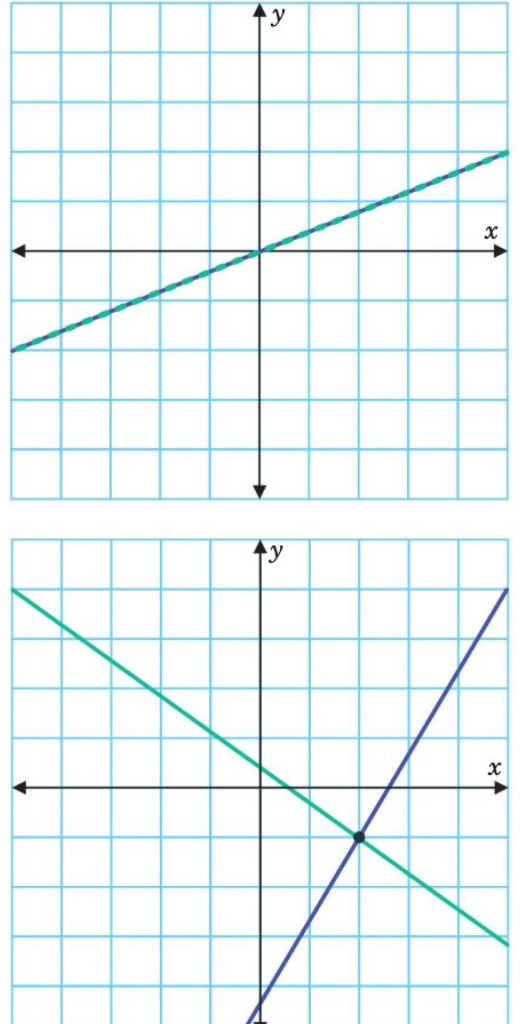
Worked Example: Graphical solution with infinite solutions

Solve the system graphically:

$1. \quad y = \frac{3}{4}x - 6$

$2. \quad 4y = 3x - 24$

Strategy: Convert equation 2 to gradient-intercept form and compare with equation 1.

Solution:

Starting with equation 2:

$4y = 3x - 24$

$y = \frac{3}{4}x - 6 \quad \text{Divide both sides by 4}$

Since equation 2 simplifies to the same form as equation 1, the two lines are identical. The graph shows that both equations represent the same line.

The system has infinitely many solutions because the lines overlap completely.

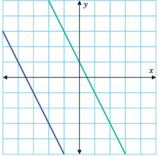
Worked Example: Graphical solution with no solution

Solve the system graphically:

$1. \quad 6x + 3y = 18$

$2. \quad 12x + 6y = 24$

Strategy: Calculate the intercepts of each equation and plot them.

Finding intercepts for equation 1:

$x$-intercept (let $y = 0$):

$6x + 3(0) = 18$

$6x = 18$

$x = 3$

$y$-intercept (let $x = 0$):

$6(0) + 3y = 18$

$3y = 18$

$y = 6$

The intercepts for equation 1 are $(3, 0)$ and $(0, 6)$.

Finding intercepts for equation 2:

$x$-intercept (let $y = 0$):

$12x + 6(0) = 24$

$12x = 24$

$x = 2$

$y$-intercept (let $x = 0$):

$12(0) + 6y = 24$

$6y = 24$

$y = 4$

The intercepts for equation 2 are $(2, 0)$ and $(0, 4)$.

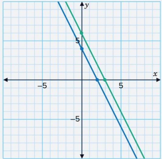
The graphs of the equations never intersect, so there is no solution to this system.

Why? Converting both equations to gradient-intercept form reveals they have the same gradient but different $y$-intercepts, confirming the lines are parallel.

Worked Example: Flower shop problem

Gordiano made two trips to a flower shop. On his first trip, he purchased 4 roses and 4 sunflowers for $12. The following day, he went back and purchased 12 roses and 8 sunflowers for $16.

The situation can be represented by:

$1. \quad 4x + 4y = 12$

$2. \quad 12x + 8y = 16$

where $x$ = cost per rose and $y$ = cost per sunflower.

Part a) Graph the system

Strategy: Define variables, then convert equations to gradient-intercept form.

Based on the problem, $x$ represents the cost per rose and $y$ represents the cost per sunflower.

Converting equation 1:

$4x + 4y = 12$

$4y = 12 - 4x \quad \text{Subtract } 4x \text{ from both sides}$

$y = -x + 3 \quad \text{Divide both sides by 4}$

Converting equation 2:

$12x + 8y = 16$

$8y = 16 - 12x \quad \text{Subtract } 12x \text{ from both sides}$

$y = -\frac{3}{2}x + 2 \quad \text{Divide both sides by 8}$

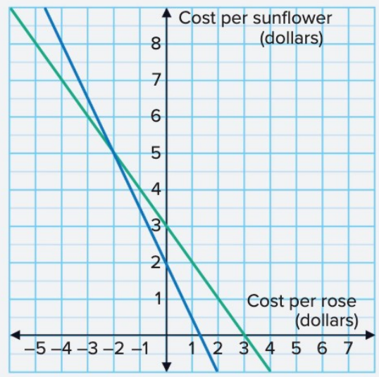
Part b) Interpret the solution

Each equation models the relationship between the total cost and the quantities of each type of flower purchased on a given day.

The solution to the system is $(-3, 6)$, which suggests a cost of -$3 per rose and $6 per sunflower.

A negative cost is not realistic in this context, so the solution is non-viable.

This indicates that at least one of the per-item costs must have been different on the two days.

Worked Example: Coin jar problem

Bixia is saving 20 cent and 5 cent pieces in a jar. She has a total of $10.50 in 90 coins.

Part a) Write a system of equations

Strategy: Use the information to create two equations - one for the total number of coins, another for the total dollar amount.

Let:

• $x$ = number of 20 cent pieces
• $y$ = number of 5 cent pieces

The system is:

$1. \quad x + y = 90$

$2. \quad 0.20x + 0.05y = 10.50$

Verification: Equation 1 represents the total number of coins. Equation 2 represents the total dollar value, where $0.20x$ is the value of all 20 cent pieces and $0.05y$ is the value of all 5 cent pieces.

Part b) Graph the system

Strategy: Find the intercepts and use them to determine appropriate scales for the axes.

For equation 1:

$x$-intercept (let $y = 0$):

$x + 0 = 90$

$x = 90$

$y$-intercept (let $x = 0$):

$0 + y = 90$

$y = 90$

For equation 2:

$x$-intercept (let $y = 0$):

$0.20x + 0.05(0) = 10.50$

$0.20x = 10.50$

$x = 52.5$

$y$-intercept (let $x = 0$):

$0.20(0) + 0.05y = 10.50$

$0.05y = 10.50$

$y = 210$

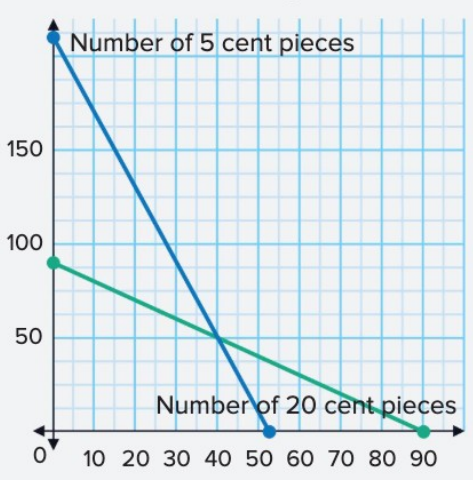
Part c) Interpret the solution

The solution to the system is $(40, 50)$. Since $x$ represents the number of 20 cent pieces, Bixia has 40 twenty-cent pieces. Since $y$ represents the number of 5 cent pieces, she has 50 five-cent pieces.

Worked Example: Rectangle perimeter problem

The length of a rectangle is 3 metres less than twice its width. If the perimeter is 48 metres, determine the length.

Strategy: Define variables and build a system of equations.

Let $l$ = length in metres and $w$ = width in metres.

From the problem:

• Length equals 3 metres less than twice the width: $l = 2w - 3$
• Perimeter equals sum of twice the length and twice the width: $2l + 2w = 48$

System:

$1. \quad l = 2w - 3$

$2. \quad 2l + 2w = 48$

Solving using substitution:

$2l + 2w = 48$

$2(2w - 3) + 2w = 48 \quad \text{Substitute } l = 2w - 3$

$4w - 6 + 2w = 48 \quad \text{Apply distributive property}$

$6w - 6 = 48 \quad \text{Combine like terms}$

$6w = 54 \quad \text{Add 6 to both sides}$

$w = 9 \quad \text{Divide both sides by 6}$

Now find $l$:

$l = 2w - 3$

$l = 2 \times 9 - 3 \quad \text{Substitute } w = 9$

$l = 15 \quad \text{Simplify}$

The length of the rectangle is 15 metres.

Worked Example: Test scores problem

Verna noticed that the sum of her Chemistry and English test scores was 128, and their difference was 16. She scored higher on her Chemistry test.

Part a) Write a system of equations

Let $x$ = Chemistry test score and $y$ = English test score.

Since the Chemistry score is higher, the difference is $x - y$ to get a positive result.

$1. \quad x + y = 128$

$2. \quad x - y = 16$

Note: There are constraints based on typical test scores: $0 \leq x \leq 100$ and $0 \leq y \leq 100$.

Part b) Solve the system

Strategy: Since the equations have the same coefficient of $y$ with opposite signs, add the equations to eliminate $y$.

$$\begin{array}{rcl} x + y &=& 128 \

• \quad x - y &=& 16 \ \hline 2x + 0y &=& 144 \end{array}$$`

Eliminate the $y$ term:

`$2x = 144$

$x = 72 \quad \text{Divide both sides by 2}$

Substitute $x = 72$ into equation 1:

$x + y = 128$

$72 + y = 128 \quad \text{Substitute } x = 72$

$y = 56 \quad \text{Subtract 72 from both sides}$

Verna scored 72 on her Chemistry test and 56 on her English test.

Alternative method: Since both equations also have the same coefficient of $x$ with the same sign, the system could be solved by subtracting one equation from the other to find $y$ first.

Part c) Does the solution make sense?

Yes. Assuming the tests were out of 100, both 72 and 56 are valid test scores to obtain.

Worked Example: Bakery break-even problem

A bakery produces cakes at a cost of $25 each with a daily fixed cost of $200. Each cake sells for $30.

Part a) Write expressions for daily cost and revenue

Strategy: Define $x$ as the number of cakes. Write cost as fixed plus variable cost per cake, and revenue as price per cake times quantity.

For the cost, the fixed value is $200 plus $25 per cake:

$C = 200 + 25x$

For the revenue, the value is $30 per cake:

$R = 30x$

Constraint: $x \geq 0$ (integers), since cakes are sold in whole units.

Part b) Determine the break-even point algebraically

Strategy: Equate cost and revenue ($C = R$), solve for $x$, then find the corresponding cost and revenue.

$C = R \quad \text{Equate } C \text{ to } R$

$200 + 25x = 30x \quad \text{Substitute the values}$

$200 = 5x \quad \text{Subtract } 25x \text{ from both sides}$

$x = 40 \quad \text{Divide both sides by 5}$

Substitute $x = 40$ into $R$:

$R = 30x$

$= 30 \times 40 \quad \text{Substitute } x = 40$

$= \$1200 \quad \text{Evaluate}$

The break-even point is $(40, 1200)$, meaning selling 40 cakes results in cost and revenue both equal to $1200.

Since $x = 40$ is an integer and satisfies $x \geq 0$, it is viable and confirms the break-even point.

Part c) Calculate the profit if 50 cakes are sold

Strategy: Calculate revenue and cost for $x = 50$, then subtract cost from revenue.

For the revenue:

$R = 30x$

$= 30 \times 50 \quad \text{Substitute } x = 50$

$= \$1500$

For the cost:

$C = 200 + 25x$

$= 200 + 25 \times 50 \quad \text{Substitute } x = 50$

$= 200 + 1250$

$= \$1450$

For the profit:

$\text{Profit} = \text{Revenue} - \text{Cost}$

$= 1500 - 1450$

$= \$50$

The bakery makes a $50 profit when selling 50 cakes.