Logarithmic Graphs Revision Notes for HSC SSCE Mathematics Advanced

Logarithmic Graphs

Introduction to logarithmic functions

A logarithmic function has the general form $y = \log_a(x)$ , where $a$ is the base of the logarithm and must satisfy $a > 0$ and $a \neq 1$ . Understanding how to graph logarithmic functions is essential for visualising their behaviour and identifying their key characteristics. These functions are the inverse of exponential functions, which means they undo the operation of exponentiation.

infoNote

The inverse relationship between logarithmic and exponential functions is fundamental to understanding their behavior. Just as subtraction undoes addition, logarithmic functions reverse the process of exponentiation. This property will become especially important when we explore their graphical relationship later.

Key features of logarithmic graphs

Every logarithmic graph has two fundamental features that help us identify and sketch them accurately. Understanding these features will make graphing logarithmic functions straightforward.

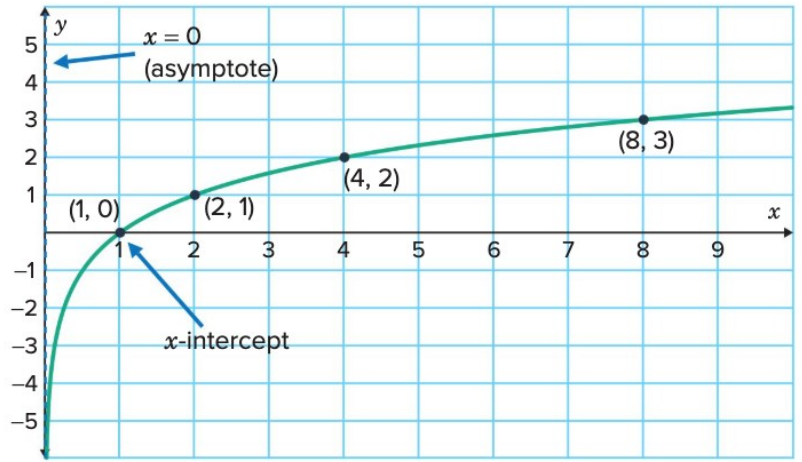
Vertical asymptote

The most important characteristic of a logarithmic graph is its vertical asymptote at $x = 0$ . This means the graph approaches the $y$ -axis but never actually touches or crosses it. As $x$ approaches zero from the right, the $y$ -values decrease towards negative infinity. This occurs because logarithms are only defined for positive input values.

x-intercept

The x-intercept of any logarithmic function $y = \log_a(x)$ always occurs at the point (1, 0). This is a universal feature regardless of the base value. We can verify this mathematically by setting $y = 0$ and solving for $x$ :

When $y = 0$ :

$0 = \log_a(x)$

Converting to exponential form:

$x = a^0$

$x = 1$

This confirms that the x-intercept is always at (1, 0) for any logarithmic function.

Domain and range

chatImportant

Critical Properties of Logarithmic Functions:

The domain of any logarithmic function is $x > 0$ , meaning the function only accepts positive input values. This explains why the vertical asymptote exists at $x = 0$ – the function cannot be evaluated at or to the left of the $y$ -axis.

The range is all real numbers, written as $y \in \mathbb{R}$ . The graph extends infinitely upward and downward, meaning logarithmic functions can output any real number value.

Additionally, there is no y-intercept for logarithmic functions because they are not defined at $x = 0$ .

Effect of base on graph shape

The base $a$ of a logarithmic function significantly affects how the graph appears. When comparing logarithmic functions with different bases, several patterns emerge.

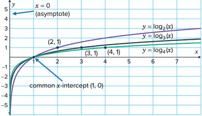
All logarithmic functions share these common features:

The x-intercept remains at (1, 0) regardless of the base
The vertical asymptote remains at x = 0 for all bases
There is no y-intercept for any base value

However, the base affects the steepness and position of the curve:

Graphs with larger bases (such as $\log_4(x)$ ) are closer to the x-axis and increase more gradually
Graphs with smaller bases (such as $\log_2(x)$ ) are further from the x-axis and increase more steeply

For example, $\log_4(x)$ is closer to the x-axis than $\log_2(x)$ . This relationship helps us predict the relative positions of logarithmic graphs without detailed calculations.

infoNote

Understanding Base Behavior:

Think of the base as controlling how "stretched" the graph appears. Larger bases create flatter, more gradual curves, while smaller bases create steeper curves. Despite these differences, all logarithmic graphs maintain the same fundamental structure – they all pass through $(1, 0)$ and have a vertical asymptote at $x = 0$ .

Worked example: Sketching logarithmic graphs

lightbulbExample

Worked Example: Sketching $y = \log_5(x)$

Let's work through a complete example of sketching a logarithmic function, labelling all important features and determining its domain and range.

Step 1: Finding the x-intercept

We begin by identifying where the graph crosses the x-axis, which occurs when $y = 0$ :

y = \log_5(x) 0 = \log_5(x) x = 5^0 x = 1

Therefore, the x-intercept is at (1, 0).

Step 2: Finding another key point

To accurately sketch the curve, we need at least one more point. A convenient choice is to use $x = 5$ (the base value):

y = \log_5(x) y = \log_5(5) y = 1

This gives us the point (5, 1), which is particularly useful because it uses the base of the logarithm.

Step 3: Completing the sketch

Now we can plot these points and sketch the logarithmic curve:

Mark the vertical asymptote at $x = 0$
Plot the x-intercept at $(1, 0)$
Plot the additional point at $(5, 1)$
Draw a smooth curve that passes through these points, approaching the asymptote as $x$ approaches zero

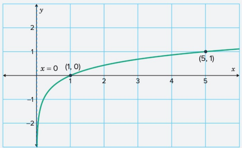
Step 4: Determining domain and range

From the completed graph, we observe that the function is only defined for positive x-values. The y-values can be any real number.

Domain: $x > 0$

Range: All real $y$ (or $y \in \mathbb{R}$ )

Exponential and logarithmic inverse relationships

Logarithmic and exponential functions have a special relationship – they are inverse functions of each other. This means that one function undoes the operation of the other.

For any base $a > 0$ where $a \neq 1$ :

The exponential function is $y = a^x$
The logarithmic function is $y = \log_a(x)$

These two functions are reflections of each other over the line $y = x$ . This reflection property is a hallmark of inverse functions.

Verifying the reflection property

We can confirm that two functions are reflections over $y = x$ by checking that key points swap coordinates. Let's examine the relationship between $y = 2^x$ and $y = \log_2(x)$ :

For the exponential function $y = 2^x$ :

The point $(0, 1)$ lies on the curve
The horizontal asymptote is at $y = 0$

For the logarithmic function $y = \log_2(x)$ :

The point $(1, 0)$ lies on the curve (notice the coordinates have swapped!)
The vertical asymptote is at $x = 0$

infoNote

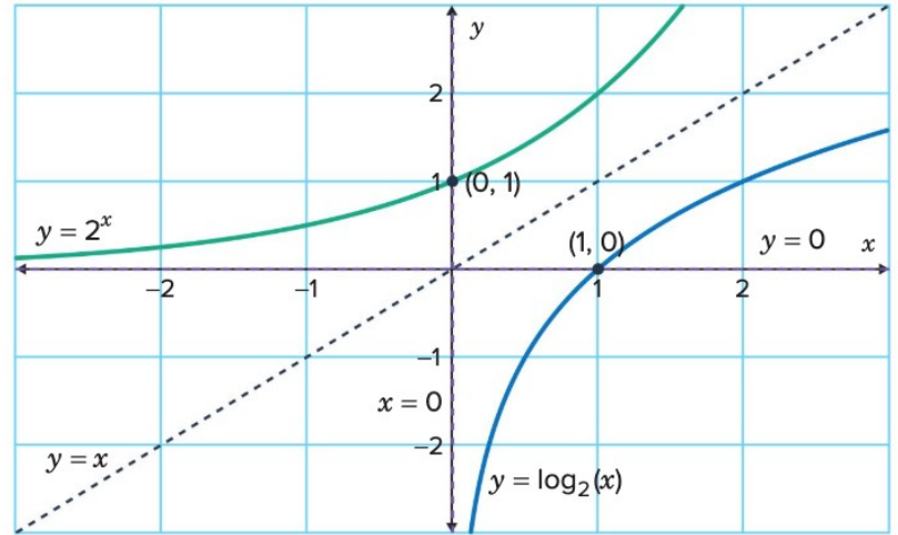
Notice how the asymptotes also reflect: the horizontal asymptote of the exponential function becomes the vertical asymptote of the logarithmic function. This symmetry is a powerful visual confirmation of their inverse relationship.

Growth comparison

When $a > 1$ , both functions are increasing, but they grow at dramatically different rates:

The exponential function $y = a^x$ grows rapidly – its values increase explosively
The logarithmic function $y = \log_a(x)$ grows slowly – its values increase gradually

This contrast in growth rates is another important distinction between these inverse functions.

Verification with base 3

lightbulbExample

Worked Example: Verifying Inverse Relationship with Base 3

Let's verify the reflection property using $y = 3^x$ and $y = \log_3(x)$ . We can check that key points confirm the reflection over $y = x$ :

Checking coordinate swaps:

For $y = 3^x$ :

Point $(0, 1)$ maps to (1, 0) on $y = \log_3(x)$

For $y = \log_3(x)$ :

Point $(1, 0)$ maps to (0, 1) on $y = 3^x$

Verifying asymptotes:

Asymptotes also confirm the reflection:

For $y = 3^x$ , the horizontal asymptote is at $y = 0$
For $y = \log_3(x)$ , the vertical asymptote is at $x = 0$

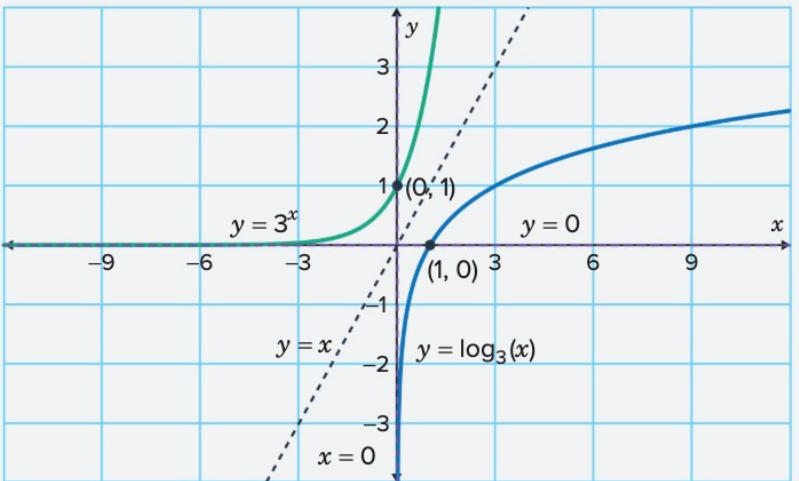
Additional verification:

We can verify with any additional point. For example, $(1, 3)$ on $y = 3^x$ maps to $(3, 1)$ on $y = \log_3(x)$ , confirming the symmetry over the line $y = x$ .

Key takeaways

bookmarkSummary

Key Points to Remember:

The logarithmic function $y = \log_a(x)$ has a vertical asymptote at x = 0 and an x-intercept at (1, 0) for any valid base.
The domain is x > 0 (positive values only) and the range is all real numbers ( $y \in \mathbb{R}$ ). There is no y-intercept.
Higher bases produce flatter curves that sit closer to the x-axis, while smaller bases produce steeper curves.
Exponential and logarithmic functions are inverse functions that reflect over the line $y = x$ . Key points $(a, b)$ on one function correspond to points $(b, a)$ on the other.
When $a > 1$ , exponential functions grow rapidly while their inverse logarithmic functions grow slowly, both increasing but at vastly different rates.

Logarithmic Graphs (HSC SSCE Mathematics Advanced): Revision Notes