The Derivative Revision Notes for HSC SSCE Mathematics Advanced

Graphical Behaviour of Functions

Introduction

The graphical behaviour of a function describes how the function changes as we move along its curve. Understanding this behaviour is crucial for analysing functions and solving real-world problems. The first derivative of a function provides valuable information about whether the function is increasing, decreasing, or stationary at any point.

infoNote

In this topic, we will explore how to use the derivative to determine the characteristics of a function's graph, find important points such as stationary points, sketch derivative graphs, and estimate derivative values using different methods.

Features of a function from its derivative

The first derivative of a function, denoted as $f'(x)$ , gives us information about the gradient of the tangent line to the curve $y = f(x)$ at any point $x$ . This gradient is the key to understanding how the function behaves.

Increasing and decreasing functions

When we examine the sign of the first derivative, we can determine whether the function is rising or falling:

If the derivative is positive at a point, the function is increasing at that point
If the derivative is negative at a point, the function is decreasing at that point
If the derivative is zero at a point, the function may have a stationary point at that point

infoNote

Let's look at two simple examples to illustrate these concepts:

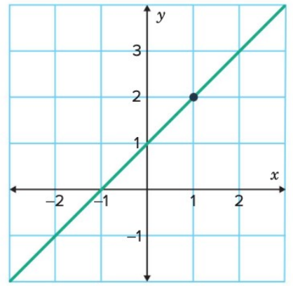
The function $y = x + 1$ is always increasing. At every point on this line, the gradient is positive. Specifically, the gradient $f'(x) = 1$ , which is always positive, confirming that the function constantly increases.

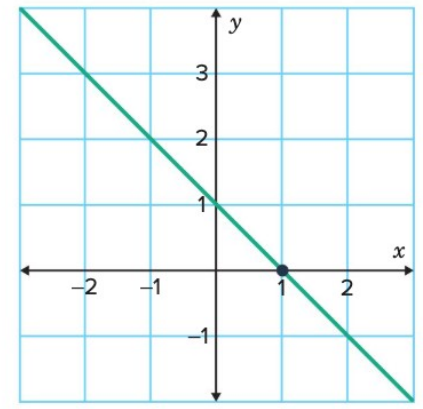
In contrast, the function $y = -x + 1$ is always decreasing. Here, the gradient $f'(x) = -1$ is always negative, indicating that the function continuously decreases as $x$ increases.

Stationary points

A stationary point is a special location on a function's graph where the tangent line is horizontal. At these points, the function momentarily stops increasing or decreasing.

chatImportant

Definition: A stationary point on the graph $y = f(x)$ of a differentiable function is a point where $f'(x) = 0$ .

A differentiable function is a function that can be differentiated at each point in its domain. This means we can find the derivative at any point along the curve.

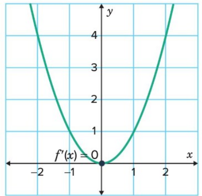
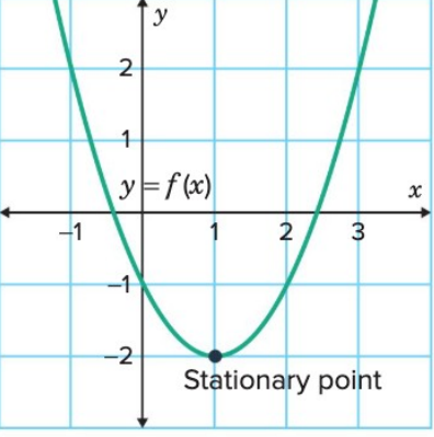
Consider the parabola $y = x^2$ . This function has a stationary point at $(0, 0)$ where the gradient $f'(x) = 0$ . At this minimum point, the tangent to the curve is perfectly horizontal.

Understanding function behaviour through derivatives

bookmarkSummary

Key Relationships Between Derivatives and Function Behaviour:

If $f'(x) > 0$ on an interval, then $f(x)$ is an increasing function on that interval
If $f'(x) < 0$ on an interval, then $f(x)$ is a decreasing function on that interval
If $f'(c) = 0$ at a point $x = c$ , then the function has a stationary point at $x = c$ , where the tangent to the curve is horizontal

These relationships allow us to analyse the behaviour of more complex functions by examining their derivatives.

Cubic functions and stationary points

The concepts of increasing, decreasing, and stationary behaviour are particularly useful when analysing polynomial functions, especially cubic functions.

What is a cubic function?

infoNote

A cubic function is a polynomial function of degree 3. It has the general form:

$f(x) = ax^3 + bx^2 + cx + d$

where $a$ , $b$ , $c$ , and $d$ are constants, and $a \neq 0$ .

Cubic functions often have interesting graphical features, including up to two stationary points (a local maximum and a local minimum) and an inflection point where the curve changes its direction of curvature.

Finding stationary points on cubic functions

To find the stationary points of any function, including cubic functions, we use the derivative. The process involves setting the derivative equal to zero and solving for $x$ .

Let's work through a detailed example to see how this works in practice.

Worked example: Finding intervals of increase and decrease

lightbulbExample

Consider the function $f(x) = x^3 - 6x^2 + 5$

a) Determine the values of $x$ for which the function is increasing or decreasing.

Strategy

Our approach will be to:

Find the derivative $f'(x)$
Set the derivative equal to zero to find stationary points
Test values of $x$ around these stationary points to determine where $f'(x)$ is positive (increasing) or negative (decreasing)

Solution

Step 1: Find the derivative

$f(x) = x^3 - 6x^2 + 5$

$f'(x) = 3x^2 - 12x$

Step 2: Find stationary points

Set $f'(x) = 0$ :

$3x^2 - 12x = 0$

Factorise:

$3x(x - 4) = 0$

Using the null factor law:

$x = 0 \text{ or } x = 4$

Step 3: Test intervals

These values divide the $x$ -axis into three intervals: $x < 0$ , $0 < x < 4$ , and $x > 4$ . We need to test a point in each interval to determine the sign of $f'(x)$ .

For $x < 0$ , test $x = -1$ :

f'(x) = 3x^2 - 12x f'(-1) = 3 \times (-1)^2 - 12 \times (-1) = 3 + 12 = 15

Since $f'(-1) > 0$ , the function is increasing for $x < 0$ .

For $0 < x < 4$ , test $x = 1$ :

f'(x) = 3x^2 - 12x f'(1) = 3 \times (1)^2 - 12 \times 1 = 3 - 12 = -9

Since $f'(1) < 0$ , the function is decreasing for $0 < x < 4$ .

For $x > 4$ , test $x = 5$ :

f'(x) = 3x^2 - 12x f'(5) = 3 \times (5)^2 - 12 \times 5 = 75 - 60 = 15

Since $f'(5) > 0$ , the function is increasing for $x > 4$ .

Conclusion: The function is increasing for $x < 0$ and $x > 4$ , and decreasing for $0 < x < 4$ .

b) Determine the coordinates of the stationary points and show them on a sketch of the function.

Strategy

We already know the $x$ -coordinates of the stationary points from part (a). We now substitute these values into the original function to find the corresponding $y$ -coordinates, then plot the points on a graph.

Solution

When $x = 0$ :

f(x) = x^3 - 6x^2 + 5 f(0) = (0)^3 - 6 \times (0)^2 + 5 = 5

When $x = 4$ :

f(x) = x^3 - 6x^2 + 5 f(4) = (4)^3 - 6(4)^2 + 5 = 64 - 6 \times 16 + 5 = 64 - 96 + 5 = -27

The coordinates of the stationary points are $(0, 5)$ and $(4, -27)$ .

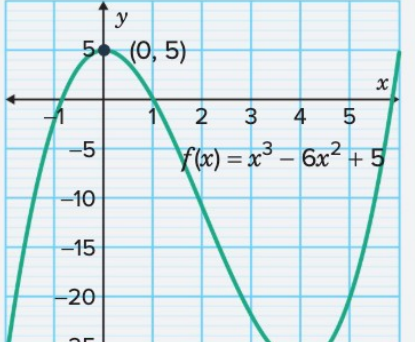
The graph confirms our analysis. The function increases up to $x = 0$ , decreases between $x = 0$ and $x = 4$ , and then increases again for $x > 4$ . The stationary points at $(0, 5)$ and $(4, -27)$ are clearly visible.

chatImportant

Key Insight:

The sign of the first derivative, $f'(x)$ , tells us whether the function is increasing, decreasing, or stationary at any given point. To find stationary points for a cubic function (or any polynomial), we calculate the derivative, set it equal to zero, and solve for $x$ .

Graphing the derivative function

We can sketch the graph of a function's derivative, $y = f'(x)$ , directly from the graph of the original function, $y = f(x)$ , by carefully observing the gradient behaviour.

Key relationships between a function and its derivative

When sketching the derivative from the original function, look for these important relationships:

infoNote

1. Stationary points become x-intercepts

Where $f(x)$ has a stationary point (horizontal tangent), the graph of $f'(x)$ will cross the $x$ -axis. This is because the gradient is zero at stationary points.

2. Increasing intervals correspond to positive derivative values

Where $f(x)$ is increasing (positive gradient), the graph of $f'(x)$ will be above the $x$ -axis, since $f'(x) > 0$ .

3. Decreasing intervals correspond to negative derivative values

Where $f(x)$ is decreasing (negative gradient), the graph of $f'(x)$ will be below the $x$ -axis, since $f'(x) < 0$ .

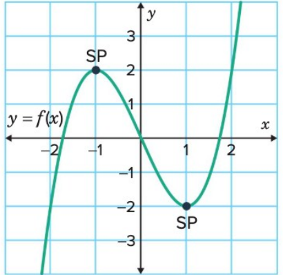
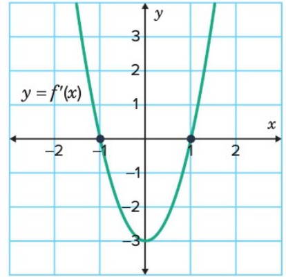
This cubic function $y = f(x)$ has two stationary points (SP) marked on the graph. These occur where the tangent line is horizontal.

The derivative $y = f'(x)$ is shown here. Notice that its $x$ -intercepts match the locations of the stationary points on the original function $f(x)$ .

Degree of the derivative

chatImportant

An important property to remember is that the degree of the derivative of a polynomial is one less than the degree of the original function. For example:

If $f(x)$ is a quadratic (degree 2), then $f'(x)$ will be linear (degree 1)
If $f(x)$ is a cubic (degree 3), then $f'(x)$ will be quadratic (degree 2)

This helps us determine the general shape of the derivative graph.

Worked example: Sketching the derivative graph

lightbulbExample

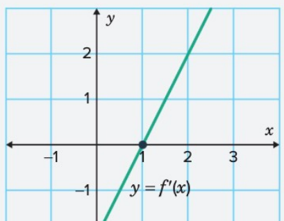
The graph of a quadratic function $y = f(x)$ is shown. Sketch the graph of its derivative, $y = f'(x)$ .

Strategy

To sketch the derivative:

Find the $x$ -coordinate of the stationary point, which will become an $x$ -intercept of $f'(x)$
Determine the intervals where $f(x)$ is decreasing and increasing to know where $f'(x)$ is negative and positive
Remember that since $f(x)$ is quadratic, $f'(x)$ will be a straight line

Solution

Step 1: Identify the stationary point

The graph of $f(x)$ has a stationary point at $x = 1$ . At this point, the gradient is zero. Therefore, the graph of $f'(x)$ must have an $x$ -intercept at $x = 1$ .

Step 2: Identify the decreasing interval

The graph of $f(x)$ is decreasing for all $x < 1$ . This means the gradient is negative in this interval. Therefore, the graph of $f'(x)$ must be below the $x$ -axis (where $f'(x) < 0$ ) for $x < 1$ .

Step 3: Identify the increasing interval

The graph of $f(x)$ is increasing for all $x > 1$ . This means the gradient is positive in this interval. Therefore, the graph of $f'(x)$ must be above the $x$ -axis (where $f'(x) > 0$ ) for $x > 1$ .

Step 4: Sketch the derivative

Combining these observations, we know that $y = f'(x)$ is a straight line that:

Passes through the point $(1, 0)$
Has a positive gradient (rises from left to right)
Is below the $x$ -axis for $x < 1$
Is above the $x$ -axis for $x > 1$

This is the graph of the derivative function $y = f'(x)$ .

bookmarkSummary

Steps for Sketching a Derivative Graph:

To sketch the graph of the derivative $y = f'(x)$ from the graph of $y = f(x)$ :

Identify the $x$ -coordinates of any stationary points on $f(x)$ . These become the $x$ -intercepts on the graph of $f'(x)$
Identify the intervals where $f(x)$ is increasing. The graph of $f'(x)$ will be above the $x$ -axis for these intervals
Identify the intervals where $f(x)$ is decreasing. The graph of $f'(x)$ will be below the $x$ -axis for these intervals
Remember that the derivative of a polynomial has a degree one less than the original function

Estimating the derivative at a point

While differentiation rules allow us to calculate the exact value of a derivative, it is sometimes useful to estimate the derivative at a specific point. This can be done using either a graphical method or a numerical method.

Graphical estimation

The graphical method involves drawing a tangent line to the curve at the point of interest and calculating the gradient of that tangent line.

infoNote

Process:

Draw the graph of the function $y = f(x)$
Identify the point $P$ where the derivative needs to be estimated
Draw a straight line that just touches the curve at point $P$ (the tangent)
Choose two distinct points on the tangent line
Use the gradient formula $m = \frac{\text{rise}}{\text{run}}$ to calculate the tangent's gradient

The gradient of the tangent line is an estimate of the derivative at that point.

Numerical estimation

The numerical method uses a formula based on the gradient of a secant line through two very close points. This provides a good approximation of the gradient of the tangent.

When we have two points that are very close together, the secant line connecting them is nearly identical to the tangent line at that location. The closer the points, the better the approximation.

chatImportant

The gradient of the secant line through $(c, f(c))$ and $(c + h, f(c + h))$ is given by:

$f'(c) \approx \frac{f(c + h) - f(c)}{h}$

where:

$f'(c)$ is the approximate derivative (gradient) at $x = c$
$h$ is a very small number (e.g., $0.01$ or $0.001$ )

The smaller the value of $h$ , the better the approximation. Digital tools such as graphing calculators can perform this calculation very efficiently.

Worked example: Estimating the derivative

lightbulbExample

Consider the function $f(x) = x^3$ where the derivative has to be estimated at $x = 1$ .

a) Estimate $f'(1)$ graphically.

Strategy

We need to sketch the graph of $y = x^3$ , draw a tangent at the point $(1, 1)$ , select another point on this tangent, and then calculate the gradient using the two points.

Solution

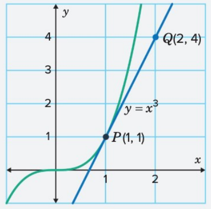
The tangent line at $P(1, 1)$ is drawn in blue. Another point on the tangent is $Q(2, 4)$ . We can now calculate the gradient.

m = \frac{y_2 - y_1}{x_2 - x_1} = \frac{4 - 1}{2 - 1} = \frac{3}{1} = 3

The graphical estimate for $f'(1)$ is $3$ .

b) Estimate $f'(1)$ numerically using a value of $h = 0.01$ .

Strategy

We use the numerical estimation formula $f'(c) \approx \frac{f(c + h) - f(c)}{h}$ with $c = 1$ and $h = 0.01$ .

Solution

$f'(c) \approx \frac{f(c + h) - f(c)}{h}$

Substitute $c = 1$ and $h = 0.01$ :

$f'(1) \approx \frac{f(1 + 0.01) - f(1)}{0.01}$

Simplify the input to the function:

$\approx \frac{f(1.01) - f(1)}{0.01}$

Apply the function rule $f(x) = x^3$ :

$\approx \frac{(1.01)^3 - (1)^3}{0.01}$

Evaluate the powers:

$\approx \frac{1.030301 - 1}{0.01}$

Evaluate the subtraction:

$\approx \frac{0.030301}{0.01}$

Evaluate the division:

$\approx 3.0301$

The numerical estimate for $f'(1)$ is $3.0301$ .

c) Find the exact value of $f'(1)$ and compare it with the estimates from parts (a) and (b). Interpret the results.

Strategy

We differentiate $f(x) = x^3$ to find $f'(x)$ , then evaluate at $x = 1$ . We can then compare this exact value with our graphical and numerical estimates to assess their accuracy.

Solution

$f(x) = x^3$

Differentiate using the power rule:

$f'(x) = 3x^2$

Substitute $x = 1$ :

f'(1) = 3 \times (1)^2 = 3

The exact value of $f'(1)$ is $3$ .

Comparison and interpretation

Graphical estimate: The graphical estimate is $3$ , which is exactly the same as the exact value. This indicates a precise tangent line approximation in this case. The simplicity of the cubic function and the carefully chosen tangent points made this method very accurate.

Numerical estimate: The numerical estimate is $3.0301$ , which is slightly higher than the exact value by $0.0301$ . This small difference arises because $h = 0.01$ is not infinitesimally small, but the estimate is still very close. The numerical method demonstrates effectiveness even with relatively small values of $h$ .

infoNote

Both estimation methods provide results close to the exact derivative. The graphical method happened to be exact in this instance due to the function's simplicity and the chosen tangent points. The numerical method's slight error highlights that smaller values of $h$ would improve accuracy, as the secant line would better approximate the tangent line.

bookmarkSummary

Methods for Estimating Derivatives:

The value of the derivative at a point on a curve can be estimated using two main methods:

Graphically: Draw a tangent to the curve at the point of interest and calculate the gradient of that tangent line using two points on the tangent.

Numerically: Use the formula $f'(c) \approx \frac{f(c + h) - f(c)}{h}$ with a very small value for $h$ (such as $0.01$ or $0.001$ ).

These methods provide approximations of the derivative, while differentiation rules give the exact value. The numerical method becomes more accurate as $h$ gets smaller, and graphing calculators can perform these calculations instantly for very precise estimates.

Remember!

bookmarkSummary

Key Points to Remember:

The first derivative $f'(x)$ tells us about the gradient of the tangent to the curve at any point. If $f'(x) > 0$ , the function is increasing; if $f'(x) < 0$ , the function is decreasing; if $f'(x) = 0$ , the function has a stationary point.
A stationary point occurs where $f'(x) = 0$ . At these points, the tangent line is horizontal. To find stationary points, set the derivative equal to zero and solve for $x$ .
For cubic functions and other polynomials, we can determine intervals of increase and decrease by finding stationary points, then testing the sign of the derivative in each interval between these points.
The graph of the derivative function $y = f'(x)$ can be sketched from the graph of $y = f(x)$ by observing where the function is increasing (derivative above $x$ -axis), decreasing (derivative below $x$ -axis), and stationary (derivative crosses $x$ -axis).
The derivative can be estimated graphically by drawing a tangent and calculating its gradient, or numerically using the formula $f'(c) \approx \frac{f(c + h) - f(c)}{h}$ with a small value of $h$ . These methods approximate the exact value obtained through differentiation.

The Derivative (HSC SSCE Mathematics Advanced): Revision Notes

Graphical Behaviour of Functions

Introduction

Features of a function from its derivative

Increasing and decreasing functions

Stationary points

Understanding function behaviour through derivatives

Cubic functions and stationary points

What is a cubic function?

Finding stationary points on cubic functions

Worked example: Finding intervals of increase and decrease

Strategy

Solution

Strategy

Solution

Graphing the derivative function

Key relationships between a function and its derivative

Degree of the derivative

Worked example: Sketching the derivative graph

Strategy

Solution

Estimating the derivative at a point

Graphical estimation

Numerical estimation

Worked example: Estimating the derivative

Strategy

Solution

Strategy

Solution

Strategy

Solution

Comparison and interpretation

Remember!

Explore HSC SSCE Mathematics Advanced Model Answers by Topics

Algebraic Techniques

Solve Equations

Introduction to Functions and Relations

Linear Functions

Quadratic and Cubic Functions

Function Properties

Functions and Relations

Trigonometry

Trigonometric Identities and Equations

Probability

Data

Introduction to Rates of Change

The Derivative

Exponential Functions

Logarithmic Functions

Transformations

Advanced Applications of Transformations

Explore HSC SSCE Mathematics Advanced Quizzes by Topics

Algebraic Techniques

Solve Equations

Introduction to Functions and Relations

Linear Functions

Quadratic and Cubic Functions

Function Properties

Functions and Relations

Trigonometry

Trigonometric Identities and Equations

Probability

Data

Introduction to Rates of Change

The Derivative

Exponential Functions

Logarithmic Functions

Transformations

Advanced Applications of Transformations

Explore HSC SSCE Mathematics Advanced Flashcards by Topics

Algebraic Techniques

Solve Equations

Introduction to Functions and Relations

Linear Functions

Quadratic and Cubic Functions

Function Properties

Functions and Relations

Trigonometry

Trigonometric Identities and Equations

Probability