Stationary Points (VCE SSCE Mathematical Methods): Revision Notes
Stationary Points
What are stationary points?
When studying the shape and behavior of a function's graph, stationary points are crucial landmarks. These are special points where the function momentarily stops increasing or decreasing - where the tangent line is perfectly horizontal.
A point on a curve is called a stationary point if the derivative at that point equals zero: .
In other words, a stationary point occurs when at .
At stationary points, the tangent line is parallel to the -axis, giving the curve a momentarily "flat" appearance at these locations. This is why the derivative (which measures the slope of the tangent) must equal zero.
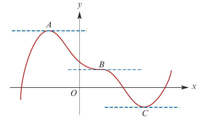
In the graph above, points , , and are all stationary points. Notice how the tangent line at each of these points (shown as dashed lines) is horizontal.
Finding stationary points
To locate the stationary points of a function, follow these steps:
- Find the derivative or
- Set the derivative equal to zero:
- Solve this equation to find the -coordinates
- Substitute each -value back into the original function to find the corresponding -coordinates
Worked example: polynomial functions
Worked Example: Finding Stationary Points of a Quadratic
Find the stationary points of .
Solution:
First, find the derivative:
Set the derivative equal to zero:
Now find the -coordinate by substituting into the original function:
Therefore, the stationary point is .
Worked example: cubic functions
Worked Example: Finding Stationary Points of a Cubic
Find the stationary points of .
Solution:
Find the derivative:
Set equal to zero:
When :
When :
The stationary points are (1, 6) and (-1, 2).
Worked example: trigonometric functions
Worked Example: Trigonometric Functions
Find the stationary points of for .
Solution:
Find the derivative:
Set equal to zero:
This occurs when:
Therefore:
Substituting these values:
- When :
- When :
- When :
- When :
The stationary points are , , , and .
Worked example: exponential functions
Worked Example: Exponential Functions
Find the stationary points of .
Solution:
Find the derivative:
Set equal to zero:
Taking natural logarithms:
When :
The stationary point is .
Worked example: logarithmic functions
Worked Example: Logarithmic Functions
Find the stationary points of for .
Solution:
Using the product rule:
Set equal to zero:
When :
The stationary point is .
Finding unknown parameters
Sometimes we need to determine unknown coefficients in a function when we're given information about stationary points or other conditions the curve must satisfy.
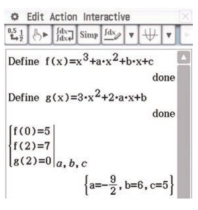
Worked Example: Finding Unknown Parameters
The curve with equation passes through the point and has a stationary point at . Find , , and .
Solution:
Since the curve passes through :
When , , so
Find the derivative:
Since there's a stationary point at , we know when :
Also, the point lies on the curve:
Multiply equation 2 by 2:
Rearranging equation 1:
Substituting into equation 2:
Therefore:
The values are: , , and .
Types of stationary points
Not all stationary points are the same. There are three main types, each with different characteristics based on how the gradient changes around the point.
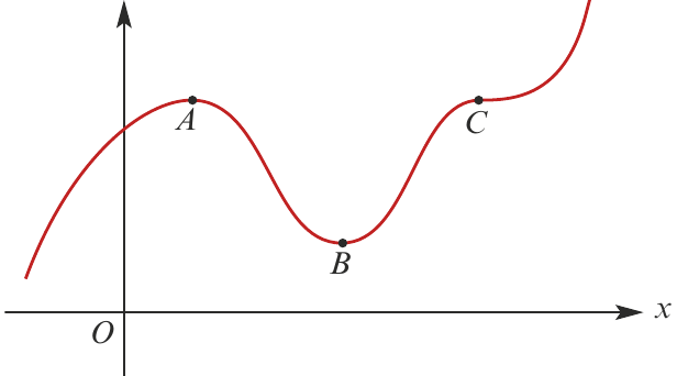
Local maximum points
A local maximum point is where the function reaches a peak in its immediate neighborhood.
At a local maximum (like point in the diagram):
- The gradient is positive immediately to the left
- The gradient is zero at the point
- The gradient is negative immediately to the right
Think of it like climbing a hill - you're going up before the summit, flat at the summit, then down after. The gradient changes from positive → zero → negative.
Local minimum points
A local minimum point is where the function reaches a valley or trough in its immediate neighborhood.
At a local minimum (like point in the diagram):
- The gradient is negative immediately to the left
- The gradient is zero at the point
- The gradient is positive immediately to the right
Think of it like walking through a valley - you're going down before the bottom, flat at the bottom, then up after. The gradient changes from negative → zero → positive.
Stationary points of inflection
A stationary point of inflection is where the function has a horizontal tangent but doesn't turn around.
At a stationary point of inflection (like point in the diagram):
- The gradient has the same sign on both sides of the point
- Either: positive → zero → positive
- Or: negative → zero → negative
The function continues in the same general direction but momentarily levels out. The key difference from turning points is that the gradient sign doesn't change.
Important terminology: Local maximum and local minimum points are collectively called turning points because the function changes direction at these points. Stationary points of inflection are NOT turning points.
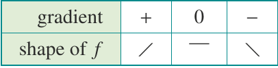
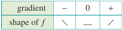
Using gradient tables to classify stationary points
A gradient table (also called a sign diagram) is a systematic way to determine what type each stationary point is. Here's how to create one:
- Find all stationary points by solving
- Test the sign of on either side of each stationary point
- Record these signs in a table
- Use the pattern to classify each point
Worked Example: Using Gradient Tables
For the function , find the stationary points and state their nature.
Solution:
Find the derivative:
Find stationary points by solving :
Calculate the -coordinates:
When :
When :
The stationary points are and .
Now test the sign of in each region:
For , try : ✓ (positive)
For , try : ✗ (negative)
For , try : ✓ (positive)
Create the gradient table:
| Shape of |
Conclusion:
- At : gradient changes from to , so there's a local maximum at
- At : gradient changes from to , so there's a local minimum at
Sketching graphs using stationary points
Stationary points are key features when sketching the graph of a function. Combined with information about axis intercepts and end behavior, they help create an accurate sketch.
Worked example: sketching an exponential function
Worked Example: Sketching an Exponential Function
Sketch the graph of .
Solution:
End behavior: As , , so
Axis intercepts: When :
The curve passes through .
Stationary points:
For stationary points:
Since for all , we need , giving .
The only stationary point is at .
Nature of stationary point: Notice that for all (it's always positive or zero).
The gradient is never negative, so the point is a stationary point of inflection.
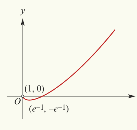
Worked example: sketching a logarithmic function
Worked Example: Sketching a Logarithmic Function
For , where , sketch the graph.
Solution:
Derivative: Using the product rule:
Solving :
Since , we need , giving .
The curve crosses the -axis at .
Stationary points: when
When :
Stationary point:
Nature: For : (gradient negative)
For : (gradient positive)
Therefore, is a local minimum.
Worked example: sketching with multiple turning points
Worked Example: Multiple Turning Points
Find the local maximum and local minimum points of where .
Solution:
Find the derivative:
Set equal to zero:
This gives us: or
Solutions in the given interval:
From :
From :
Calculate -values:
Create a gradient table:
Conclusions:
- Local maxima at and
- Local minima at and
Using CAS calculators
Modern CAS (Computer Algebra System) calculators can help verify stationary points and assist with graphing. While you need to understand the concepts, calculators can check your work.
Finding key features with a graphing calculator
For the function , a CAS calculator can:
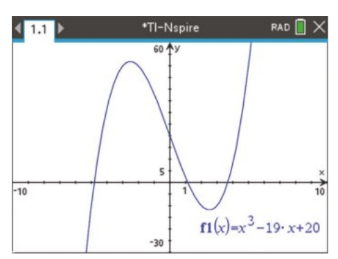
- Plot the graph in an appropriate viewing window
- Evaluate the function at specific points
- Find zeros (where the graph crosses the -axis)
- Calculate derivatives at specific points
- Locate maximum and minimum points
Example calculations:
When :
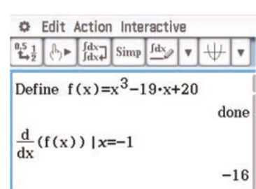
The derivative at :
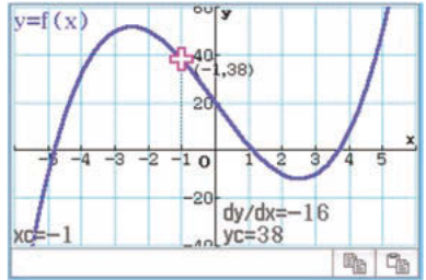
The graph shows these features clearly with the derivative value displayed at the point.
Exam tip: While calculators are helpful tools, you must be able to find and classify stationary points by hand. Use calculators to check your working, but always show full algebraic steps in exam answers.
Summary
Key Points to Remember:
-
Stationary points occur where the derivative equals zero: or
-
Three types of stationary points:
- Local maximum: gradient changes from + to 0 to -
- Local minimum: gradient changes from - to 0 to +
- Stationary point of inflection: gradient maintains sign (+ to 0 to + or - to 0 to -)
-
Use gradient tables systematically: Test the sign of on either side of each stationary point to determine its type
-
Turning points are local maxima or minima - points where the function changes direction
-
When sketching graphs, combine stationary points with axis intercepts and end behavior for a complete picture