The General Cubic Function Revision Notes for VCE SSCE Mathematical Methods

The General Cubic Function

What is a general cubic function?

A general cubic function is a polynomial of degree three that can be written in the form:

f(x) = ax^3 + bx^2 + cx + d, \text{ where } a \neq 0

This is different from the transformation form $f(x) = a(x - h)^3 + k$ that you might have seen before. Not all cubic functions can be expressed in the transformation form, which is why we need to understand the general form.

infoNote

The general cubic function allows us to work with any cubic polynomial, regardless of its shape or position on the coordinate plane. The coefficient $a$ determines whether the graph rises or falls as $x$ increases, while the other coefficients $b$ , $c$ , and $d$ affect the shape and position of the curve.

chatImportant

Why we need calculus for cubic functions:

To fully investigate cubic functions, we need calculus. This means finding exact coordinates of turning points requires techniques you'll learn later. For now, we can use CAS calculators to find these points approximately.

Shapes of cubic graphs

Cubic graphs come in a wonderful variety of shapes. Unlike quadratic graphs which all have the same basic parabola shape, cubic graphs can look quite different from one another. Here's a gallery showing some common cubic shapes:

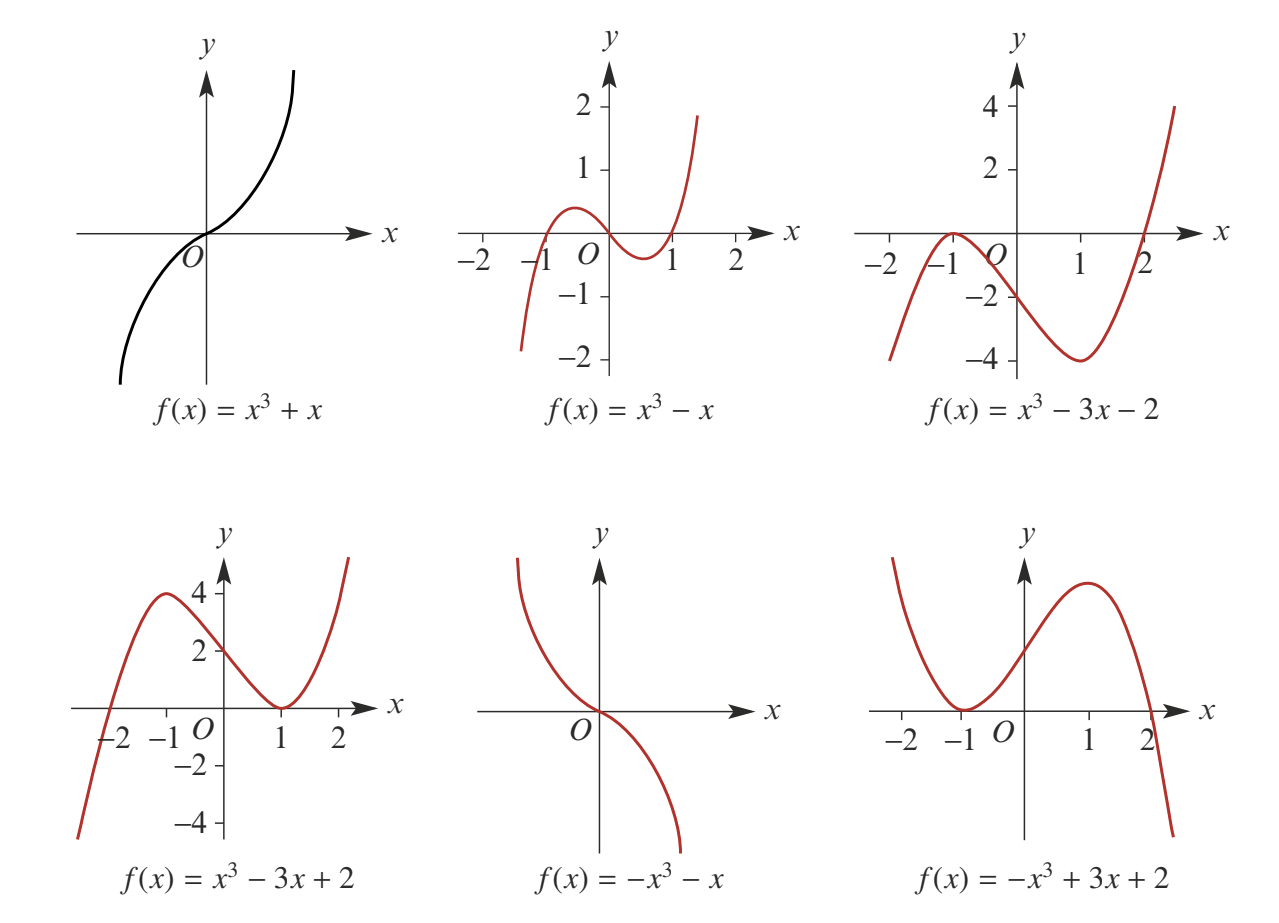
These graphs demonstrate the diversity of cubic functions. Notice how some curves are smooth and monotonic (always increasing or decreasing), whilst others have distinctive S-shapes with hills and valleys. The presence and position of turning points dramatically affects the appearance of each graph.

Key characteristics of cubic graphs

Understanding the behaviour of cubic graphs is essential for sketching them accurately. Here are the most important characteristics you need to know:

Number of x-axis intercepts

A cubic graph can cross the x-axis at one, two, or three points. This depends on how many real solutions the equation $f(x) = 0$ has. Look at the gallery above and count the x-intercepts in each graph to see this variety in action.

Stationary points

chatImportant

Not all cubic graphs have stationary points!

Not all cubic graphs have stationary points (points where the gradient is zero). For example, the graph of $f(x) = x^3 + x$ has no stationary points at all - it continuously increases without any turning points. Other cubics may have one or two stationary points, which we call local maximum and local minimum points.

When a cubic does have turning points, they are found using differential calculus. Your CAS calculator can find these coordinates for you by approximating them to decimal places.

Asymmetry of turning points

Unlike quadratic graphs, the turning points of a cubic function do not occur symmetrically between consecutive x-axis intercepts. This means you cannot find turning points simply by averaging the x-intercepts. This is another reason why we need calculus to locate them precisely.

Repeated factors

When a cubic graph has a turning point that touches the x-axis (rather than crossing it), this corresponds to a repeated factor in the factorised form of the function.

lightbulbExample

Worked Example: Identifying a Repeated Factor

The graph of $f(x) = x^3 - 3x - 2$ has a turning point at $(-1, 0)$ . This function can be factorised as:

f(x) = (x + 1)^2(x - 2)

Notice the repeated factor $(x + 1)^2$ . The exponent of 2 indicates that the graph touches the x-axis at $x = -1$ but doesn't cross it. This creates a turning point at that x-intercept.

Sign diagrams

Sign diagrams are useful tools for understanding when a cubic function is positive or negative. They help us visualise the behaviour of the function across different intervals of the x-axis.

A sign diagram is a number line that shows whether a function's output is positive $(+)$ or negative $(-)$ for different values of $x$ . For a cubic function in factorised form $f(x) = (x - \alpha)(x - \beta)(x - \gamma)$ , where $\alpha < \beta < \gamma$ , the sign diagram looks like this:

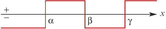
The diagram divides the number line into regions based on the x-intercepts (also called zeros or roots). In each region, we determine whether the function is positive or negative. The sign alternates as we move across each x-intercept, starting from the right-hand side.

infoNote

Creating a sign diagram:

To create a sign diagram, follow these steps:

Find all x-intercepts by solving $f(x) = 0$
Mark these values on a number line in ascending order
Test the sign of $f(x)$ in each interval between (and beyond) the intercepts
Mark each region with $+$ or $-$ accordingly

lightbulbExample

Worked Example: Creating a Sign Diagram

Let's draw a sign diagram for the cubic function $f(x) = x^3 - 4x^2 - 11x + 30$ .

Step 1: Factorise the function

From factorising, we get:

f(x) = (x + 3)(x - 2)(x - 5)

This tells us that $f(-3) = f(2) = f(5) = 0$ , so our x-intercepts are at $x = -3$ , $x = 2$ , and $x = 5$ .

Step 2: Determine the sign in each interval

Now we determine the sign of $f(x)$ in each interval:

For $x > 5$ : all three factors are positive, so $f(x) > 0$
For $2 < x < 5$ : $(x + 3)$ is positive, $(x - 2)$ is positive, but $(x - 5)$ is negative, giving $f(x) < 0$
For $-3 < x < 2$ : $(x + 3)$ is positive, but both $(x - 2)$ and $(x - 5)$ are negative, giving $f(x) > 0$
For $x < -3$ : all three factors are negative, so $f(x) < 0$

Step 3: Complete the sign diagram

Here's the completed sign diagram:

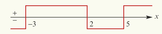
Notice how the sign alternates as we cross each x-intercept, creating a pattern of regions where the function is positive or negative.

Sketching cubic graphs with CAS calculators

When sketching cubic graphs, we often need to find the exact coordinates of turning points. Since this requires calculus, we use CAS calculators to find these coordinates approximately.

lightbulbExample

Worked Example: Sketching and Transforming a Cubic

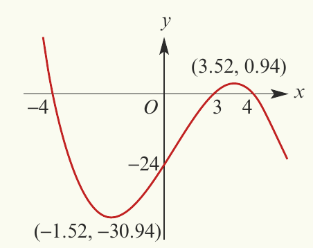
For the cubic function with rule $f(x) = -x^3 + 19x - 30$ :

Part a: Sketch the graph of $y = f(x)$ using a calculator to find the coordinates of the turning points, correct to two decimal places.

Step 1: Factorise the function

f(x) = -x^3 + 19x - 30

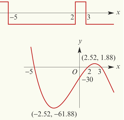
The x-axis intercepts are at $x = -5$ , $x = 2$ , and $x = 3$ .

Step 2: Find the y-axis intercept

The y-axis intercept is found by substituting $x = 0$ :

f(0) = -30

Step 3: Create the sign diagram

Here's the sign diagram for this function:

Step 4: Use CAS calculator to find turning points

Using a CAS calculator (method described below), we find the turning points:

Local maximum at $(2.52, 1.88)$
Local minimum at $(-2.52, -61.88)$

The completed sketch shows all these features clearly.

Part b: Sketch the graph of $y = \frac{1}{2}f(x - 1)$ .

Step 1: Identify the transformation

The transformation rule is:

(x, y) \to \left(x + 1, \frac{1}{2}y\right)

This represents a dilation of factor $\frac{1}{2}$ from the x-axis, followed by a translation of 1 unit to the right.

Step 2: Transform the turning points

Let's transform the turning points:

$(2.52, 1.88) \to (3.52, 0.94)$
$(-2.52, -61.88) \to (-1.52, -30.94)$

Step 3: Sketch the transformed graph

The transformed graph is shown below:

Notice how the transformation has compressed the graph vertically by half and shifted it one unit to the right.

Using a CAS calculator to find turning points

To find the coordinates of turning points (local maxima and minima) on your calculator:

infoNote

TI-Nspire Method:

Enter the function in a Graphs page
Set an appropriate viewing window using menu > Window/Zoom > Window Settings
Use menu > Trace > Graph Trace or menu > Analyse Graph > Maximum or Minimum
In Graph Trace mode, move the tracing point using arrow keys or by typing a specific x-value
When the point reaches a local minimum or maximum, it displays the type of turning point
Press enter to paste the coordinates to the graph
Press esc to exit

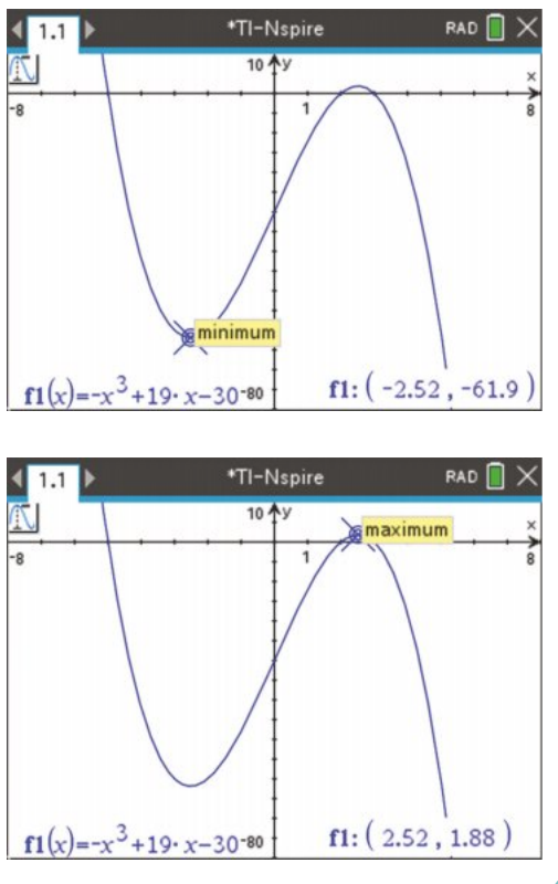
The calculator screens show how to locate both the minimum and maximum points of the cubic function we sketched earlier.

infoNote

Alternative Method: Analyse Graph

If you use Analyse Graph instead of Graph Trace:

Select the lower bound by moving to the left of the turning point and clicking
Select the upper bound by moving to the right of the turning point and clicking
The calculator will then calculate and display the coordinates

This method is particularly useful when you want to find a specific turning point in a particular region of the graph.

Summary

bookmarkSummary

Key Points to Remember:

General form: A general cubic function is written as $f(x) = ax^3 + bx^2 + cx + d$ where $a \neq 0$
Intercepts: Cubic graphs can have one, two, or three x-axis intercepts
Turning points: Not all cubic graphs have stationary points - some increase (or decrease) continuously. When turning points exist, there can be zero, one, or two of them
Repeated factors: If a turning point lies on the x-axis, the function has a repeated factor (power of 2) at that x-intercept
Sign diagrams: Create sign diagrams by marking x-intercepts on a number line and determining whether the function is positive or negative in each interval
Finding turning points: Use your CAS calculator's graphing features to find approximate coordinates of local maxima and minima, as calculus is needed to find them exactly

The General Cubic Function (VCE SSCE Mathematical Methods): Revision Notes