Objectives of Government Economic Policy (AQA A-Level Economics): Revision Notes
Objectives of Government Economic Policy
What are macroeconomic policy objectives?
Macroeconomics examines the economy as a whole rather than focusing on individual markets or firms. While microeconomics looks at specific questions like 'what determines the price of bread?', macroeconomics addresses broader questions such as 'what determines the average price level of all goods and services?' and 'what determines the rate of inflation?'. These questions about output levels, consumption, investment, and trade lie at the heart of macroeconomics.
A policy objective is a target or goal that the government aims to achieve or 'hit'. Since the Second World War (1939-45), governments in mixed economies like the UK have generally pursued the same broad set of objectives.
The Four Main Macroeconomic Policy Objectives:
- Economic growth: Achieving economic growth and improving living standards and levels of economic welfare
- Full employment: Creating and maintaining full employment or low unemployment
- Price stability: Limiting or controlling inflation, or achieving some measure of price stability
- Balance of payments: Attaining a satisfactory balance of payments, usually defined as avoiding an external deficit which might create an exchange rate crisis
Understanding these objectives is essential because they guide government economic policy and help us evaluate how well an economy is performing.
Economic growth
Economic growth refers to an increase in the real output of goods and services produced by an economy over time. We need to distinguish between two types of economic growth: short-run and long-run.
Short-run and long-run economic growth
Short-run economic growth occurs when there are unemployed resources (including labour) or 'slack' in the economy. This type of growth involves moving from a point inside the economy's production possibility frontier to a point on the frontier. Short-run growth is also called economic recovery because it represents the economy using resources that were previously idle.
Long-run economic growth, by contrast, results from an outward movement of the production possibility frontier itself. This means the economy's productive capacity has expanded, allowing it to produce more goods and services than before. Long-run growth requires increases in the quantity or quality of resources (such as a larger workforce, better technology, or more capital equipment).
Think of short-run growth as using what you already have more efficiently (like using idle factory capacity), while long-run growth means expanding what you have (like building new factories or developing new technology).
Real GDP versus nominal GDP
When measuring economic growth, economists use real GDP rather than nominal GDP.
Nominal GDP is the sum of all goods and services produced in the economy over a period of time (typically one year), measured at the current market prices. The problem with nominal GDP is that it can increase simply because prices have risen, even if the actual quantity of output hasn't changed.
Real GDP adjusts for price changes or inflation. It measures all the goods and services produced in an economy in real terms, giving us an accurate picture of changes in the total output of the economy. When we talk about economic growth, we always mean growth in real GDP, not nominal GDP.
Key Formula:
The relationship between real and nominal GDP can be expressed as:
Understanding recession
A recession occurs when real national output declines for a sustained period. In the UK and many other countries, a recession is officially defined as six months or more of negative economic growth (declining real GDP).
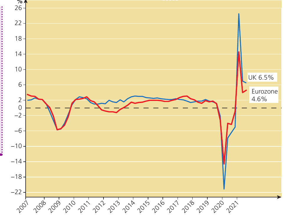
The chart above shows the year-on-year economic growth rates in the UK and the eurozone from 2007 to 2021. Several important patterns emerge from this data:
- Both the UK and eurozone experienced severe recessions following the 2008-09 financial crisis, with growth rates falling to around
- There was a continuous but slow recovery in the UK after 2009, with growth rates generally between and until 2019
- The eurozone entered a second recession in 2012
- Both economies experienced dramatic falls in GDP during the Covid-19 pandemic in 2020, with growth rates plunging to around
- A sharp V-shaped recovery followed in 2021, though growth rates varied between the UK () and eurozone ()
The volatility in recent years has been much greater than in previous decades, largely due to the Covid-19 lockdowns and the uncertainty created by the pandemic.
Case study: The Great Depression in the 1930s
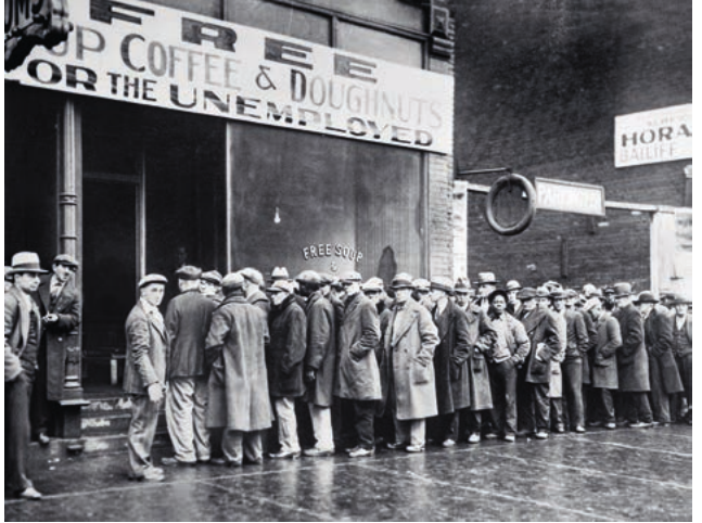
A depression is a more severe form of recession, representing a longer and deeper economic downturn. The most famous example is the Great Depression of the 1930s.
The 1920s was a period of growing national prosperity in the USA. However, the Great Depression, which began in 1929-30, was far steeper and more protracted in the USA than in other industrial countries. Consider these stark statistics:
- The US unemployment rate rose higher and remained higher longer than in any other developed country
- US real GDP fell by 9.4% in 1930 and the unemployment rate climbed from to
- In 1931, real GDP fell by another 8.5% and unemployment rose to
- By 1932, real GDP had fallen in the USA by 31% since 1929 and over 13 million Americans had lost their jobs
- The US economy began recovering in 1934, with real GDP rising by and unemployment falling to
The Great Depression demonstrated that market forces alone do not automatically deliver full employment and economic growth. This event fundamentally changed economic thinking and led to the development of Keynesian economics, which argues for government intervention to manage the economy.
Calculating mean and median values
Economists often work with data sets showing economic performance across different regions or time periods. Two important measures for summarising such data are the mean (average) and the median (middle value).
Worked Example: Calculating Mean and Median GVA Growth Rates
The table below shows the percentage change in gross value added (GVA) per head in UK regions for 2019:
| Region | % change in GVA per head |
|---|---|
| London | 3.8 |
| South East | 3.5 |
| East of England | 2.9 |
| West Midlands | 1.7 |
| East Midlands | 2.7 |
| Yorkshire and Humber | 3.0 |
| South West | 2.7 |
| North West | 2.7 |
| North East | 2.5 |
| Scotland | 3.0 |
| Wales | 2.1 |
| Northern Ireland | 2.0 |
Step 1: Calculate the mean
Add up all the values and divide by the number of regions:
The mean value is 2.72% (to 2 decimal places).
Step 2: Calculate the median
First arrange the values from highest to lowest:
3.8, 3.5, 3.0, 3.0, 2.9, 2.7, 2.7, 2.7, 2.5, 2.1, 2.0, 1.7
Since there are 12 values (an even number), the median is the average of the sixth and seventh numbers:
Interpretation: The median value of 2.7% is slightly lower than the mean, suggesting that a few regions with higher growth rates (particularly London and the South East) are pulling the average up.
Full employment and unemployment
Full employment is one of the four main policy objectives, but economists define it in different ways.
Two definitions of full employment
Beveridge's Definition
In 1944, a famous White Paper on employment policy, written by William Beveridge (an economist at the London School of Economics, who later became Lord Beveridge), effectively committed modern governments to achieving full employment. Beveridge defined full employment as occurring when unemployment falls to 3% of the labour force.
However, many free-market economists regard Beveridge's 3% definition as too arbitrary and lacking theoretical justification.
Free-Market Definition
Free-market economists favour a different definition of full employment. For them, full employment occurs when the aggregate labour market reaches its market-clearing real-wage rate. At this point, the number of workers willing to work equals the number of workers whom employers wish to hire. In other words, the supply of labour equals the demand for labour.
According to this view, there will always be some unemployment in the economy simply because it's constantly changing, with jobs disappearing and new jobs being created. Beveridge's definition accepts this reality by allowing for 3% unemployment even at 'full employment'.
Methods of measuring unemployment in the UK
The UK has used two main methods to measure unemployment: the claimant count and the Labour Force Survey.
The claimant count measures unemployment according to the number of people claiming unemployment-related benefits (previously called Jobseeker's Allowance, now largely replaced by Universal Credit). This measure has been dropped by the UK government as an official measure of unemployment because it's increasingly a poor proxy for overall unemployment levels.
The Labour Force Survey (LFS) is now the official measure of unemployment. This is a quarterly sample survey of households in the UK that collects information about respondents' personal circumstances and their labour market status over a period of one to four weeks.
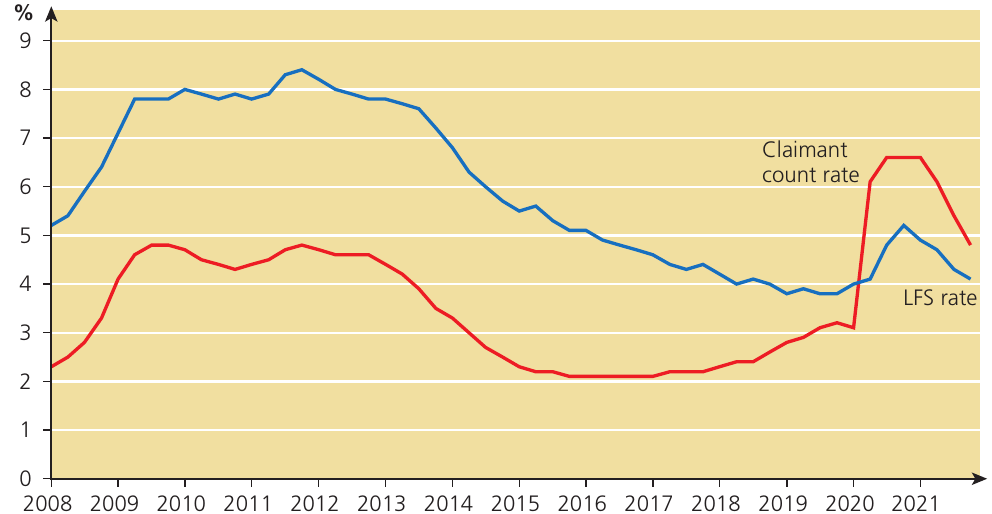
The chart above shows how these two measures have differed over time from 2008 to 2021:
- The claimant count rate started higher (around in 2008), peaked at about in 2012, then declined steadily to roughly by 2019 before rising again
- The LFS rate began at in 2008, rose to plateau around from 2009-2013, then dropped significantly to approximately from 2014-2019
- During the Covid-19 pandemic in 2020-2021, the LFS rate spiked dramatically to before declining slightly, while the claimant count also rose significantly
After 2013, the claimant count measure began to include recipients of Universal Credit, making the link between the two measures less comparable. This is especially true after the start of Covid-19, when many more households relied on Universal Credit and the furlough scheme between April 2020 and September 2021.
How the ONS measures unemployment
The Office for National Statistics (ONS) uses the Labour Force Survey as the basis for official unemployment figures. Here's how it works:
- Each quarter, the LFS covers 100,000 people in 40,000 households chosen randomly by postcode
- This represents about one in 600 of the total population
- The results are weighted to give an estimate that reflects the entire population
- The survey has a very large sample size compared to opinion polls (which often survey around 1,000 people)
- Even so, there is always a margin of uncertainty, typically around plus or minus 3% for the unemployment level
To count as unemployed in the LFS, people must say they are not working, are available for work, and have either looked for work in the past four weeks or are waiting to start a new job they have already obtained. Someone who is out of work but doesn't meet these criteria counts as 'economically inactive'.
Claimant Count vs LFS
The claimant count is published monthly and derives from administrative data (Jobseeker's Allowance and Universal Credit claimants recorded by Jobcentre Plus). While this makes it available more quickly than the LFS measure, it doesn't suffer from sampling limitations, and it can be broken down to local level, it's now considered a narrower measure of unemployment. Many people who are out of work are not eligible for Jobseeker's Allowance, so the claimant count is usually much lower than the LFS measure. Additionally, unlike the LFS, the claimant count doesn't use internationally agreed definitions.
Price stability
Price stability means maintaining a low and predictable rate of inflation. This is now considered one of the most important macroeconomic objectives.
What is inflation?
Inflation is a general rise in average prices (a rise in the price level) across the economy. It's important not to confuse inflation with a change in the price of a particular good or service. Individual prices rise and fall all the time in a market economy, reflecting changes in demand, supply, preferences, and costs. Inflation occurs only when most prices are rising by some degree across the whole economy.
A change in the price of one good may lead to a change in the measured rate of inflation, particularly if spending on that item makes up a significant fraction of total consumer spending. However, inflation is fundamentally about the general price level, not individual prices.
Related concepts: deflation and disinflation
Deflation is a continuing tendency for the average price level to fall. True deflation (a falling average price level) is called deflation. In 2009, during the economic downturn, there were fears that the inflation rate would become negative, leading to deflation.
Disinflation occurs when the rate of inflation is falling but is still positive. Make sure you don't confuse deflation with disinflation. During 2022, inflation began to rise quickly, significantly above the official target. By autumn 2022, the inflation rate had risen close to and was expected to increase to just below . This was the highest UK inflation rate since 1990.
Don't Confuse These Terms!
- Inflation: Prices are rising (e.g., inflation rate of )
- Disinflation: Prices are still rising, but at a slower rate (e.g., inflation falls from to )
- Deflation: Prices are falling (e.g., inflation rate of )
Achieving price stability versus controlling inflation
Achieving absolutely stable prices means having a zero annual rate of inflation, with the average price level neither rising nor falling from year to year. Although a zero rate of inflation has occasionally been achieved, it's extremely rare.
Much more usually, in the UK at least, controlling inflation means achieving a low inflation rate rather than absolute price stability. For most of the last two decades, successive UK governments have aimed to achieve a 2% inflation rate. Until 2022, the inflation rate was either slightly above or slightly below this official target.
Price indices: CPI and RPI
A price index is an index number showing the extent to which a price, or a 'basket' of prices, has changed over a month, quarter or year, in comparison with the price(s) in a base year.
The UK uses price indices to measure the rate of consumer price inflation. The dominant price index is now the Consumer Prices Index (CPI). The CPI calculates the average price increase of a basket of 700 different consumer goods and services. The government uses the CPI for setting the inflation rate target which the Bank of England tries to hit. The CPI has also been used for indexation of welfare benefits, though in recent years some state benefits were frozen as part of the Conservative government's austerity policy.
Before 2011, the Retail Prices Index (RPI) was also used to measure consumer price inflation. The RPI is calculated in a slightly different way to the CPI.
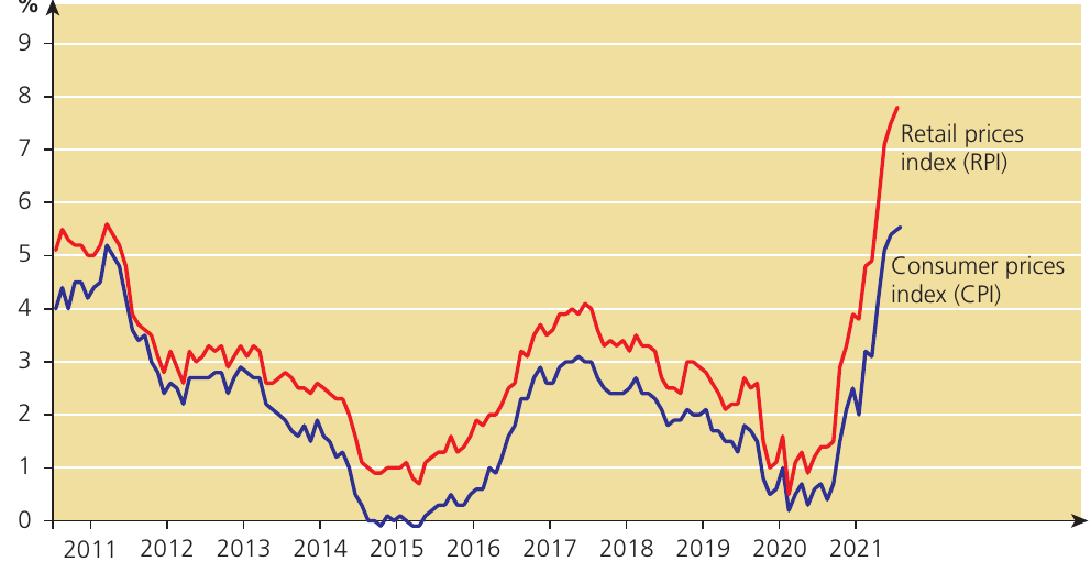
The chart above shows changes in the RPI and CPI inflation rates in the UK from January 2011 to January 2022. Notice that:
- Both measures generally move together, showing similar trends
- RPI is usually higher than CPI
- Both started around - in 2011
- Both fell to near zero in 2015
- Both rose again before falling to around - in 2020
- Both increased sharply from 2021, reaching - by 2022
In March 2018, the national statistician at the ONS stated:
"Overall, RPI is a very poor measure of general inflation, at times greatly overestimating and at other times underestimating changes in prices and how these changes are experienced. In 2013, the RPI lost its status as a National Statistic. Our position on the RPI is clear: we do not think it is a good measure of inflation and discourage its use."
Until 2011, the state pension increased each year in line with changes in the RPI. The government then replaced this with the CPI link, which has generally been more favourable to the government than to pensioners, as the chart shows. RPI inflation has usually been higher than CPI inflation.
The declining usage of the RPI as a measure of inflation has been accompanied by the growing use of other measures:
- 'Core' inflation is calculated by removing volatile items such as food and fuel from the CPI measure
- 'Headline' inflation (currently measured by changes in the CPI) may be temporarily influenced by factors that are mainly short-term in nature
- 'Underlying' inflation is measured by trying to eliminate the inflationary 'noise' created by such temporary price fluctuations
In this sense, 'underlying' inflation and 'core' inflation are much the same thing.
Calculating real values from nominal values
Understanding the relationship between nominal and real values is essential for economic analysis.
Worked Example: Calculating Real GDP Growth
Question: In Ruritania between 2022 and 2023, the rate of price inflation was and the rate of increase of nominal GDP was . What was the rate of increase of real GDP?
Solution: We use the equation:
Inserting the numbers:
Interpretation: This tells us that even though nominal GDP increased by , real GDP actually fell by 2% because prices rose faster than nominal output.
Calculating the rate of real economic growth
Worked Example: Calculating Real Economic Growth from Price-Adjusted Data
The table below shows nominal GDP and price levels for 2022 and 2023:
| Year | Nominal GDP ($ billion) | Price level |
|---|---|---|
| 2022 | 1,270 | 100 |
| 2023 | 1,410 | 108 |
Step 1: Calculate real GDP in 2023
To calculate the level of real GDP in 2023, we need to adjust for the price increase:
Step 2: Calculate the economic growth rate
Interpretation: This shows that real economic growth was 2.8%, which is much lower than the nominal GDP growth rate of [].
A satisfactory balance of payments
The balance of payments measures the flows of money into and out of an economy crossing national boundaries over a particular time period, usually a month, quarter or year.
The current account
An important part of the balance of payments is called the current account. The current account measures all the currency flows into and out of a country in a particular time period in payment for exports and imports of goods and services, together with primary and secondary income flows.
The current account contains two main sections: the money value of exports (domestically produced goods or services sold to residents of other countries), and the money value of imports (goods or services produced in other countries and sold to residents of this country).
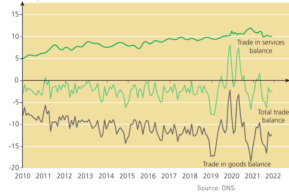
The chart above shows changes in the UK's balances of trade in goods and services, and total trade, from 2010 to 2021. Several key patterns emerge:
- Trade in services balance (dark green line) has consistently been positive, ranging from around to
- Trade in goods balance (dark blue line) has consistently been negative, between and
- Total trade balance (light green line) has fluctuated near zero, sometimes positive and sometimes negative
- There was notable volatility around 2019-2020, with dramatic dips in both goods and total trade balance
Balance of trade: deficit and surplus
Changes in exports and imports over the period 2010 to 2021 make up the balance of trade. If the money value of imports exceeds the money value of exports, there is a balance of trade deficit. If the money value of imports is less than the money value of exports, there is a balance of trade surplus.
Achieving balance on the current account of the balance of payments is one of the macroeconomic objectives. However, the word 'satisfactory' can be interpreted in different ways:
- Some people assume a satisfactory balance of payments occurs only when the government achieves the biggest possible current account surplus (when exports exceed imports by the greatest amount)
- However, a country can enjoy a trading surplus only if at least one other country suffers a trading deficit
- It's mathematically impossible for all countries to have a current account surplus at the same time
Therefore, most economists take the view that a 'satisfactory' balance of payments is a situation in which the current account is in equilibrium (balanced), or when there is a small surplus or a small but sustainable deficit.
Components of the current account
The current account includes more than just trade in goods and services. There are also primary and secondary income flows. These include:
- Income from investments abroad
- Wages and salaries earned by residents working abroad or foreign workers in the UK
- Transfer payments such as foreign aid and contributions to international organisations
Understanding all four sections of the current account is essential for analysing the causes of a surplus or deficit on this part of the balance of payments.
Other macroeconomic objectives
Governments may also pursue additional macroeconomic objectives beyond the four main ones.
Balanced budget and budget deficit
A balanced budget is achieved when government spending equals government revenue (). A budget deficit occurs when government spending exceeds government revenue ().
After the 2008-09 recession, the budget deficit (where government spending exceeds revenue from tax) increased significantly. The reduction of this deficit became a very important macroeconomic objective for the UK government until 2015 when, although the deficit remained (albeit a smaller deficit), other priorities emerged.
The deficit rose again to very high levels in 2021 as a direct result of the massive increase in government spending related to the Covid-19 pandemic. This included economic support measures such as the furlough scheme, as well as increases in health and social care spending. There was also a sharp fall in taxation revenue as incomes and spending fell significantly. However, the reduction of this deficit was not a priority in 2021, as it had been ten years earlier.
Income distribution and equity
Another macroeconomic objective is achieving a more equitable or fairer distribution of income. In recent years, the opposite has been the case: after the 2008-09 recession, income inequalities widened, although they were actually slightly narrower by 2021.
Governments have various policy objectives beyond just the four main ones, and these additional objectives can also create conflicts and trade-offs with the primary objectives.
Macroeconomic policy conflicts
Economists often argue that it's difficult, if not impossible, for a government to 'hit' all its desired macroeconomic objectives at the same time. When they can't achieve all objectives simultaneously, policy-makers often settle for the lesser goal of 'trading off' between policy objectives.
Trade-offs between policy objectives
A trade-off exists when two or more desirable objectives are mutually exclusive. Although it may be impossible to achieve two desirable objectives at the same time (e.g. zero inflation and full employment), policy-makers may be able to choose an acceptable combination lying between the extremes, such as inflation and unemployment.
This is different from a policy conflict.
Policy conflicts
A policy conflict occurs when two policy objectives cannot both be achieved at the same time: the better the performance in achieving one objective, the worse the performance in achieving the other.
Main UK Policy Conflicts
Over the years, UK macroeconomic policy has been influenced and constrained by four significant conflicts between policy objectives:
- Between the internal policy objectives of full employment and growth and the external objective of achieving a satisfactory balance of payments (or possibly supporting a particular exchange rate)
- Between achieving full employment and controlling inflation
- Between increasing the rate of economic growth and achieving a more equal distribution of income and wealth
- Between higher living standards now and higher living standards in the future (an example of an 'intertemporal' conflict — a conflict 'across time')
Short-run versus long-run policy conflicts
Most economists agree that these policy conflicts and trade-offs pose considerable problems for governments in the economic short run, defined as a period in macroeconomics extending just a few years into the future.
However, there is much less agreement about whether they need be significant in the long run — a period extending many years into the future. Pro-free-market economists often argue that if appropriate (and successful) supply-side policies are implemented, the main objectives of macroeconomic policy are compatible with each other and not in conflict in the long run.
Understanding Economic Time Periods
The short run and long run in macroeconomics are used more loosely than in microeconomics:
- The macroeconomic 'short run' may extend to about three years into the future, with the 'long run' being any period longer than that
- A period known as the 'medium term' is sometimes identified, perhaps covering 18 months to three years into the future, separating the short run and the long run
This matters because different groups of economists have different beliefs about the exact timescales of the short-run and long-run periods. If an economic problem that economists assume will resolve itself in the long run actually takes many decades to resolve, some economists may think this is justification for not attempting to solve the problem at all. Other economists may be more willing to intervene and solve problems if they think the long run might be a significantly long time away.
As the famous economist John Maynard Keynes is reported to have said: "In the long run we are all dead." This quote seeks to explain why governments should intervene in the macroeconomy rather than wait until the long run when problems may resolve themselves.
How the importance of different macroeconomic policy objectives has changed over time
The order in which the four main objectives of macroeconomic policy were listed at the beginning of this chapter shows a broadly Keynesian ranking of priorities.
The Keynesian era (1950s-1979)
In the Keynesian era, which extended roughly from the 1950s to 1979, UK governments implemented Keynesian macroeconomic policies. They believed that economic policy should be used to achieve full employment, economic growth, and a generally acceptable or fair distribution of income and wealth. These were the prime policy objectives, which had to be achieved in order to increase human happiness and economic welfare — the ultimate policy objective.
Controlling inflation and achieving a satisfactory balance of payments were regarded as intermediate objectives, or possibly as constraints. An unsatisfactory performance in controlling inflation or the balance of payments could prevent the attainment of full employment and economic growth.
The pro-free-market era (1980s onwards)
In the early 1980s, things changed. A new government in 1979, with Margaret Thatcher becoming prime minister, meant that UK governments were now pro-free market rather than Keynesian. In the 1970s, inflation had threatened to escalate out of control, and in response UK governments placed control of inflation in the top position as a policy objective, relegating full employment to a lower position in the ranking of macroeconomic policy objectives.
Since then, UK governments have continued to give much more attention to the need to control inflation. Indeed, in 1993, the Conservative chancellor Norman Lamont stated that high unemployment was a 'price well worth paying' for keeping inflation under control. This view was echoed in 1998 when, under a Labour government, the governor of the Bank of England argued that 'job losses in the north were an acceptable price to pay for curbing inflation in the south'. These statements reflect the pro-free-market view that, in order to maintain a high and sustainable level of employment, inflation must first be brought under control.
Recent developments
The long and deep recession which hit the UK (and many other countries) in 2008 led to a partial revision of this view. This was reinforced by lockdown-induced downturns of 2020 and 2021 (which technically may not actually have been recessions). For various reasons explained in later chapters, inflation was thought to have been successfully controlled and was kept close to its target rate for much of the period between 2012 and 2021.
The rapid rise in the inflation rate in 2022 was considered to have been caused by factors outside the government's control, namely:
- Rapid rises in energy prices
- Oil price increases
- Shortages and disruptions to supply chains caused by the Covid-19 pandemic (though others blamed Brexit and the war in Ukraine for some of these disruptions)
Recent UK macroeconomic policy has been dominated by a combination of 'loose' monetary policy (very low interest rates) and 'tight' fiscal policy (cutting government spending in an effort to reduce the size of the budget deficit).
It is also worth noting that, despite a rapid increase in the UK's balance of payments deficit on current account, achieving a balance of payments equilibrium has not been regarded by recent governments as an important policy objective. All this may, of course, change in the future.
The growth of Keynesian economics
Although the A-level specification only requires you to know about trends and developments in the economy over the 15 years before you sit the examination, understanding the nature of modern macroeconomics requires some knowledge of what was happening in the UK and world economies in the 1920s and 1930s.
Free-market economics in the 1920s and 1930s
Most economists at the time, especially those in UK and American universities, were free-market economists who believed that, in a competitive market economy, market forces would automatically deliver full employment and economic growth. Governments needed to have a macroeconomic policy, but it was generally believed that the policy should be restricted to maintaining 'sound money' deemed necessary for a stable price level, and possibly to maintaining a fixed exchange rate.
However, the problem was that in the UK economy of the 1920s and in the wider world economy (especially the USA) in the 1930s, free-market forces did not deliver full employment and economic growth. Instead, unregulated market forces seemed to have produced economic stagnation and mass unemployment.
The most prominent event of the time was the Great Depression, which began in 1929 and lasted until the late 1930s. Unemployment rose in 1933 to almost in the USA, and in 1931 to in the UK. Regional unemployment in towns such as Jarrow in northeast England was as high as , though London, the southeast, and the Midlands fared much better.
Keynes's response
Free-market economists responded to the Great Depression by arguing that markets were not to blame for persistent large-scale unemployment. Instead, they believed that mass unemployment was caused by institutional factors, such as the power exercised by trade unions, which prevented markets from operating freely. In the free-market view, wage cuts were necessary to 'price the unemployed into jobs'. But trade unions resisting wage cuts prevented this from happening.
In the late 1920s, John Maynard Keynes, who started his academic career as an economist in the free-market tradition, began to change his views on the main cause of unemployment. In response to an accusation of inconsistency, Keynes is reported to have said: 'When the facts change, I change my mind — what do you do, sir?'
Keynes believed that orthodox free-market economic theory failed to explain how the whole economy works, and that a better and more general theory was needed to explain mass unemployment. Keynes created his new theory in 1936 with the publication of his great book The General Theory of Employment, Interest and Money, commonly referred to as Keynes's General Theory.
Keynes's General Theory marks the beginning of modern macroeconomics. For over a generation until about 1979, Keynesian economics was macroeconomics, and macroeconomics was Keynesian economics. In the three decades after the Second World War, Keynesianism became the new economic orthodoxy in the UK, the Netherlands, and the Scandinavian countries. Economic policy in the USA also eventually became Keynesian, with the Republican president, Richard Nixon, famously stating in 1971 that 'we are all Keynesians now'.
Key Points to Remember:
-
The four main macroeconomic policy objectives are: economic growth, full employment (or low unemployment), price stability (or low inflation), and a satisfactory balance of payments.
-
Economic growth can be short-run (using idle resources to move towards the production possibility frontier) or long-run (expanding the production possibility frontier itself). Real GDP, not nominal GDP, is the correct measure of economic growth.
-
Full employment has two definitions: Beveridge's 3% unemployment rate definition, and the free-market definition of the market-clearing wage rate. The UK officially measures unemployment using the Labour Force Survey (LFS).
-
Price stability means controlling inflation, typically aiming for the UK government's 2% target. The Consumer Prices Index (CPI) is the official measure of inflation. Remember to distinguish between inflation (rising prices), deflation (falling prices), and disinflation (falling rate of inflation but still positive).
-
Balance of payments records currency flows in and out of a country. A satisfactory balance of payments typically means the current account is in equilibrium or has a small, sustainable surplus or deficit. The balance of trade is the difference between the value of exports and imports.
-
Policy conflicts and trade-offs arise when achieving one objective makes it harder to achieve another. These conflicts are generally more significant in the short run than in the long run. Pro-free-market economists argue that appropriate supply-side policies can make objectives compatible in the long run.
-
Historical context matters: The Keynesian era prioritized full employment and growth, while the pro-free-market era from the 1980s onwards prioritized controlling inflation. Recent policy has been dominated by low interest rates and fiscal restraint.