Mixed-Strategy Games Revision Notes for AQA A-Level Further Maths

Mixed-Strategy Games

What are mixed-strategy games?

In game theory, not all games have a stable solution (also called a saddle point). When you analyze a game using the maximin and minimax approaches, you may find that the maximum of the row minima does not equal the minimum of the column maxima. This indicates that no pure-strategy equilibrium exists.

A mixed-strategy game occurs when players cannot gain an advantage by consistently choosing the same strategy. In these situations, the best approach is for each player to randomize their strategy choices according to carefully calculated probabilities. This prevents the opponent from predicting their moves and exploiting a fixed pattern.

infoNote

When player A always plays their play-safe strategy, player B can take advantage of this predictability by switching to a different strategy. To prevent exploitation, player A should play different strategies at random, but with specific probabilities that maximize their expected payoff.

For example, if player A always plays their play-safe strategy, player B can take advantage of this predictability by switching to a different strategy. To prevent this, player A should play different strategies at random, but with specific probabilities that maximize their expected payoff.

Checking for stable solutions

Before using mixed strategies, you must first verify that the game has no stable solution. Use the following method:

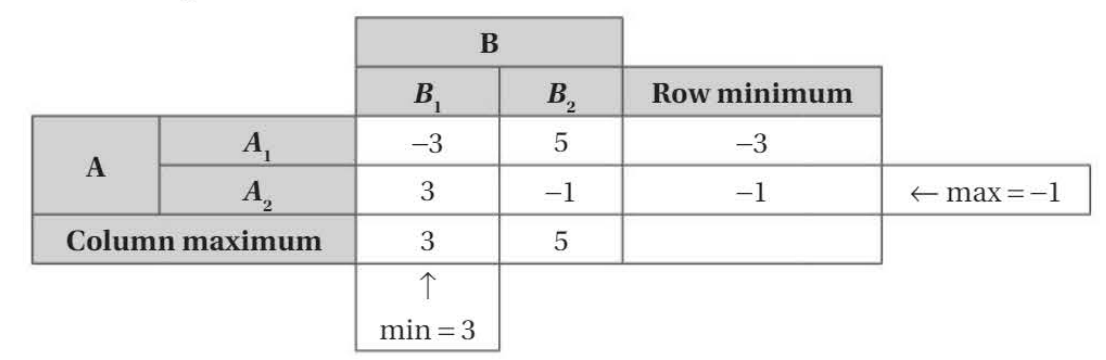
Step 1: Calculate the row minimum for each of player A's strategies (the worst outcome if A plays that row).

Step 2: Find the maximum of the row minima - this is A's play-safe value.

Step 3: Calculate the column maximum for each of player B's strategies (the worst outcome for B in each column).

Step 4: Find the minimum of the column maxima - this is B's play-safe value.

Step 5: If these values are equal, a stable solution exists. If not, you need mixed strategies.

lightbulbExample

Checking for Stable Solutions

In the example above, the max of row minima is $-1$ , but the min of column maxima is $3$ .

Since $-1 \neq 3$ , there is no stable solution, so mixed strategies are required.

Expected value and expected payoff

The concept of expectation or expected payoff is fundamental to analyzing mixed-strategy games. The expected payoff represents the average outcome you can expect over many plays of the game.

chatImportant

Definition of Expected Payoff

If payoffs $x_1, x_2, ..., x_n$ occur with probabilities $p_1, p_2, ..., p_n$ , the expectation or expected (mean) payoff $E(x)$ is given by:

$E(x) = x_1p_1 + x_2p_2 + ... + x_np_n = \sum_{i=1}^{n} x_ip_i$

This formula tells you to multiply each possible payoff by its probability, then sum all these products.

lightbulbExample

Expected Value Calculation

Suppose you play a game where:

The probability of winning is $\frac{1}{4}$
If you win, you get $10
If you lose, you pay $5

Your expected payoff per game is:

$E(x) = 10 \times \frac{1}{4} + (-5) \times \frac{3}{4} = 2.50 + (-3.75) = -\$1.25$

This means that on average, you expect to lose $1.25 per game. The negative value indicates this is not a favourable game for you.

Finding optimal mixed strategies for player A

When a game has no stable solution, you need to find the optimal probability distribution for each player's strategies. Let's work through the method for player A (the row player).

Method:

Step 1: Let player A play strategy $A_1$ with probability $p$ and strategy $A_2$ with probability $(1-p)$ .

Step 2: Let $v$ represent the value of the game (A's expected payoff).

Step 3: For each of player B's strategies, calculate player A's expected payoff:

If B plays $B_1$ : Expected payoff = (payoff for $A_1$ vs $B_1$ ) $\times p$ + (payoff for $A_2$ vs $B_1$ ) $\times (1-p)$
If B plays $B_2$ : Expected payoff = (payoff for $A_1$ vs $B_2$ ) $\times p$ + (payoff for $A_2$ vs $B_2$ ) $\times (1-p)$

Step 4: The value of the game cannot exceed these expected payoffs, giving constraints:

$v \leq$ expected payoff if B plays $B_1$
$v \leq$ expected payoff if B plays $B_2$

Step 5: Player A wants to maximize $v$ subject to these constraints. This is a linear programming problem that can be solved graphically.

Step 6: Plot the constraint lines on a graph with $p$ on the horizontal axis and $v$ on the vertical axis.

Step 7: The maximum value of $v$ occurs where the constraint lines intersect (at the lowest point of the feasible region).

Step 8: Solve the simultaneous equations to find $p$ and $v$ .

lightbulbExample

Worked Example: Finding Player A's Optimal Strategy

Consider this game:

	$B_1$	$B_2$
$A_1$	2	-1
$A_2$	-2	3

This game has no stable solution (you should verify this).

Let A play $A_1$ and $A_2$ with probabilities $p$ and $(1-p)$ .

Step 1: Calculate expected payoffs

If B plays $B_1$ , A's expected payoff is: $2p + (-2)(1-p) = 2p - 2 + 2p = 4p - 2$

If B plays $B_2$ , A's expected payoff is: $(-1)p + 3(1-p) = -p + 3 - 3p = 3 - 4p$

Step 2: Set up constraints

Player A needs to maximize $v$ subject to:

$v \leq 4p - 2$
$v \leq 3 - 4p$

Step 3: Find intersection

The maximum occurs where $4p - 2 = 3 - 4p$ :

8p = 5

p = \frac{5}{8}

Therefore, A should play $A_1$ with probability $\frac{5}{8}$ and $A_2$ with probability $\frac{3}{8}$ .

Step 4: Calculate value

The value of the game is: $v = 4 \times \frac{5}{8} - 2 = \frac{20}{8} - 2 = \frac{1}{2}$

Finding optimal mixed strategies for player B

The process for finding player B's optimal strategy is similar, but there's an important point to remember: the payoff matrix shows player A's payoffs, so from B's perspective, these payoffs are negative.

chatImportant

Key Point for Player B's Strategy

The value of the game to player B is $-v$ (the negative of the value to player A).

When calculating B's expected payoffs, remember that the payoffs shown in the matrix are from A's perspective, so you need to consider the negative of these values for B.

Method for player B:

Step 1: Let player B play strategy $B_1$ with probability $q$ and strategy $B_2$ with probability $(1-q)$ .

Step 2: For each of player A's strategies, calculate player B's expected payoff (remember to use negative values):

If A plays $A_1$ : B's expected payoff
If A plays $A_2$ : B's expected payoff

Step 3: Player B wants to maximize their value, which means maximizing $(-v)$ , equivalent to minimizing $v$ .

Step 4: Set up constraints: $-v \leq$ B's expected payoff for each of A's strategies

Step 5: Find where the constraint lines intersect to determine optimal $q$ .

lightbulbExample

Worked Example: Finding Player B's Optimal Strategy

Using the same game as before:

	$B_1$	$B_2$
$A_1$	2	-1
$A_2$	-2	3

Let B play $B_1$ and $B_2$ with probabilities $q$ and $(1-q)$ .

Step 1: Calculate expected costs

If A plays $A_1$ , B's expected payoff is: $-2q + 1(1-q) = -2q + 1 - q = 1 - 3q$

If A plays $A_2$ , B's expected payoff is: $2q + (-3)(1-q) = 2q - 3 + 3q = 5q - 3$

Step 2: Set up constraints

For B to maximize $-v$ , we need:

$-v \leq 1 - 3q$ , so $v \geq 3q - 1$
$-v \leq 5q - 3$ , so $v \geq -5q + 3$

Actually, from B's perspective, if A plays $A_1$ : B's expected payoff = $(-2) \times q + (1) \times (1-q) = -2q + 1 - q = 1 - 3q$

Following the standard approach: Player B wants to minimize the value to A.

If A plays $A_1$ , B's expected cost is: $3 \times q + (-5) \times (1-q) = 8q - 5$

So $v \geq 8q - 5$ , meaning $8q - 5 \leq v$

If A plays $A_2$ , B's expected cost is: $(-3) \times q + 1 \times (1-q) = 1 - 4q$

So $v \geq 1 - 4q$ , meaning $1 - 4q \leq v$

Step 3: Find optimal strategy

The optimal strategy occurs when these are equal:

8q - 5 = 1 - 4q

12q = 6

q = \frac{1}{2}

So B should play $B_1$ and $B_2$ each with probability $\frac{1}{2}$ .

The value of the game to B is: $8 \times \frac{1}{2} - 5 = 4 - 5 = -1$

This equals $-v$ as expected.

Solving larger payoff matrices

When dealing with larger matrices (such as 2×3, 3×2, or even larger), there's an important principle that simplifies the problem:

chatImportant

Key Principle for Larger Matrices

For a 2×n game: The column player will only use two of their $n$ available strategies in the optimal solution. The other strategies will give the row player a greater payoff and should be avoided.
For an n×2 game: The row player will only use two of their $n$ available strategies in the optimal solution.

This means you can reduce the problem to a 2×2 game by identifying which two strategies each player should use, then solving as before.

lightbulbExample

Worked Example: A 2×3 Game

Find the optimal strategies for players in this game:

	$B_1$	$B_2$	$B_3$
$A_1$	4	2	-1
$A_2$	-3	-2	5

The game has no stable solution (verify this yourself).

Step 1: Set up probabilities

Let A play $A_1$ and $A_2$ with probabilities $p$ and $(1-p)$ .

Step 2: Calculate expected payoffs for each B strategy

If B plays $B_1$ : Expected payoff = $4p + (-3)(1-p) = 4p - 3 + 3p = 7p - 3$

If B plays $B_2$ : Expected payoff = $2p + (-2)(1-p) = 2p - 2 + 2p = 4p - 2$

If B plays $B_3$ : Expected payoff = $(-1)p + 5(1-p) = -p + 5 - 5p = 5 - 6p$

Step 3: Set up constraints

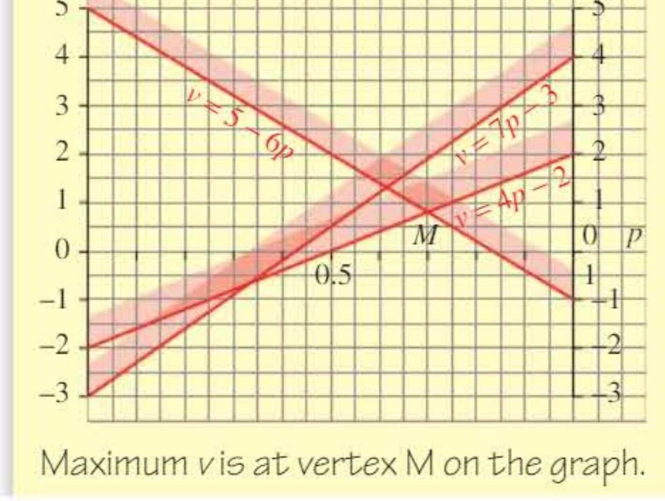
A needs to maximize $v$ subject to:

$v \leq 7p - 3$
$v \leq 4p - 2$
$v \leq 5 - 6p$

Step 4: Find intersection

Plotting these on a graph, the maximum $v$ occurs at the intersection of $v = 4p - 2$ and $v = 5 - 6p$ :

4p - 2 = 5 - 6p

10p = 7

p = 0.7

So A plays $A_1$ and $A_2$ with probabilities 0.7 and 0.3.

The value of the game is: $v = 4 \times 0.7 - 2 = 2.8 - 2 = 0.8$

Step 5: Determine which strategies B uses

Notice that the line $v = 7p - 3$ passes above the intersection point, so B should not play $B_1$ (as A's payoff would be greater than 0.8).

B will play only $B_2$ and $B_3$ with probabilities $q$ and $(1-q)$ . Following the same process as before (from B's perspective), you can find that $q = 0.6$ , so B plays $B_2$ and $B_3$ with probabilities 0.6 and 0.4.

infoNote

When solving larger matrices, always identify which constraint lines form the intersection point. Any strategy whose constraint line lies above (for player A) or below (for player B) the intersection should not be used in the optimal solution.

Strategy for solving two-player zero-sum games

Here's a systematic approach to solve any two-player zero-sum game:

Step 1: If necessary, construct the payoff matrix from the problem description.

Step 2: Use dominance to reduce the matrix as much as possible.

Step 3: Find the play-safe strategies and check whether the game has a stable solution (saddle point).

Step 4: For mixed-strategy games, find the constraints on $v$ (the value of the game) in terms of the probability or probabilities of playing the various strategies.

Step 5: Solve the resulting linear programming problem to find the optimal strategies and the value of the game. This can be done graphically (for 2×2, 2×n, or n×2 games) or algebraically.

Step 6: Answer the question in context, interpreting your results in terms of the original problem.

infoNote

This systematic approach works for all two-player zero-sum games. The key is to always check for a stable solution first before attempting to find mixed strategies - many students waste valuable exam time finding mixed strategies when a pure strategy equilibrium exists.

Exam tips and common errors

chatImportant

Critical Exam Tips

Tip 1: Always check for a stable solution first. Many students waste time finding mixed strategies when a pure strategy equilibrium exists.

Tip 2: When finding player B's optimal strategy, remember that the payoffs in the matrix are from A's perspective. You need to consider the negative of these values for B.

Tip 3: For graphical solutions, the optimal point is where constraint lines intersect. Make sure you're finding the correct intersection - the maximum for A (lowest point of upper bounds) or maximum of negative for B.

Tip 4: Probabilities must sum to 1. If you're told A plays $A_1$ with probability $p$ , then A plays $A_2$ with probability $(1-p)$ for a 2×2 game.

Tip 5: The value of the game to A should equal the negative of the value to B. Use this as a check on your work.

chatImportant

Common Mistakes to Avoid

Common Error: Forgetting to simplify expected payoff expressions. Always collect like terms:

$2p - 3(1-p) = 2p - 3 + 3p = 5p - 3$ , not $2p - 3 + 3p$ .

Common Error: Using the wrong intersection point on the graph. For player A maximizing $v$ , you want the lowest point of the upper envelope of constraint lines.

Common Error: In larger matrices, trying to use all strategies. Remember: in a 2×n game, the column player uses only 2 strategies in the optimal solution.

Remember!

bookmarkSummary

Key Points to Remember:

A mixed-strategy game occurs when there is no stable solution - the maximum of row minima does not equal the minimum of column maxima.
Expected payoff formula: $E(x) = \sum(\text{payoff} \times \text{probability})$ - multiply each outcome by its probability and sum the results.
Finding optimal strategies: Set up probability variables, calculate expected payoffs against each opponent strategy, express constraints on the game value $v$ , then solve the linear programming problem graphically or algebraically.
For larger matrices: In a 2×n game, the column player uses only 2 of their n strategies. In an n×2 game, the row player uses only 2 of their n strategies. This simplifies the problem significantly.
Value check: The value of the game to player A should equal the negative of the value to player B (since it's a zero-sum game). Use this as a verification of your solution.

Mixed-Strategy Games (AQA A-Level Further Maths): Revision Notes