Games as Linear Programming Problems (AQA A-Level Further Maths): Revision Notes
Games as Linear Programming Problems
Introduction to zero-sum games
A zero-sum game is a competitive situation between two players where one player's gain is exactly equal to the other player's loss. The total payoff for both players combined always sums to zero.
In game theory, we represent these games using a pay-off matrix, which shows the outcomes for different strategy combinations. By convention, the matrix displays payoffs from the row player's (player A) perspective.
The pay-off matrix structure:
- Rows: Representing player A's strategies (A₁, A₂, A₃, etc.)
- Columns: Representing player B's strategies (B₁, B₂, B₃, etc.)
- Entries: The payoff to player A for each combination of strategies
All values shown are gains for the row player - positive numbers mean A wins, negative numbers mean A loses (B wins).
When games do not have a stable solution with pure strategies, we need to find optimal mixed strategies using linear programming and the simplex method.
Play-safe strategies
A play-safe strategy is the approach that guarantees the best outcome in the worst-case scenario.
For the row player (A):
- Find the minimum value in each row (worst outcome for each of A's strategies)
- Select the strategy with the maximum of these minimums (maximin strategy)
For the column player (B):
- Find the maximum value in each column (worst outcome for each of B's strategies, since B wants to minimise A's gain)
- Select the strategy with the minimum of these maximums (minimax strategy)
The play-safe strategy ensures a player gets at least a certain payoff, regardless of what the opponent does. It represents a conservative approach that protects against the worst possible outcome.
Stable solutions and pure strategy games
A game has a stable solution when:
When this condition is met, the game has a pure strategy game solution. Both players will consistently use their play-safe strategies, and neither player benefits from changing strategy.
If the maximum of row minima does NOT equal the minimum of column maxima, the game has no stable solution and requires a mixed strategy, where players randomly choose between strategies according to optimal probability distributions.
Expected payoff
When players use mixed strategies, we need to calculate the expected payoff (or expected value).
Expected pay-off formula:
If payoffs occur with probabilities , then:
where:
- is the expected payoff
- are the possible payoffs
- are the corresponding probabilities
- The probabilities must satisfy: and all
Calculating Expected Payoff with Mixed Strategies
Suppose player A plays strategy A₁ with probability and strategy A₂ with probability , while player B plays strategy B₁.
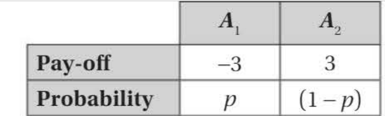
The expected payoff is:
Similarly, if player B plays strategy B₂:
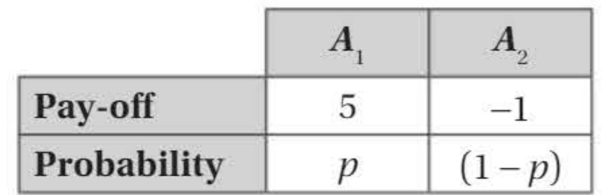
The expected payoff is:
The value of the game, , cannot be more than either expected payoff, so:
Converting games to linear programming problems
When a game has no stable solution, we solve it by converting it to a linear programming problem.
Step 1: Check for negative entries
The simplex method requires all variables to be non-negative. If the pay-off matrix contains negative entries, add a constant to every entry to make them all non-negative.
Critical step: After solving the problem, you must subtract this constant from the final value to obtain the true game value. Forgetting this step is a common mistake!
Step 2: Set up the linear programming formulation
Let player A use strategies A₁, A₂, ..., Aₙ with probabilities .
Objective function:
where is the value of the game (A's expected profit).
Constraints:
For each of player B's strategies, A's expected payoff must be at least :
- If B plays B₁:
- If B plays B₂:
- And so on for all of B's strategies
Probability constraints:
Step 3: Introduce slack variables
Convert the inequality constraints to equations by introducing slack variables (, , , etc.):
Slack variables transform inequalities into equations, which is required for the simplex algorithm. Each inequality constraint gets its own slack variable, which must also be non-negative.
Step 4: Apply the simplex algorithm
Create a simplex tableau and perform row operations until all coefficients in the objective row are non-negative.
Worked example 1: solving a 3×2 game
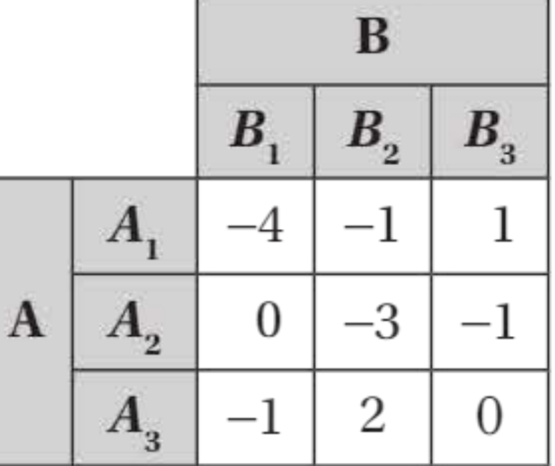
Worked Example: Solving a 3×2 Zero-Sum Game Using the Simplex Method
Problem: Use the simplex method to solve this zero-sum game and find the optimal strategy for players A and B, and the value of the game.
Solution:
Step 1: Add 2 to each entry to make all entries non-negative.
Step 2: Let A play A₁, A₂, and A₃ with probabilities , , and .
The linear programming formulation is:
Maximise
subject to
Step 3: Introduce slack variables and set up the initial tableau:
The initial simplex tableau is:
| P | v | p₁ | p₂ | p₃ | s | t | u | Value | Row |
|---|---|---|---|---|---|---|---|---|---|
| 1 | -1 | 0 | 0 | 0 | 0 | 0 | 0 | 0 | R1 |
| 0 | 1 | -3 | -2 | -1 | 1 | 0 | 0 | 0 | R2 |
| 0 | 1 | 0 | -1 | -2 | 0 | 1 | 0 | 0 | R3 |
| 0 | 0 | 1 | 1 | 1 | 0 | 0 | 1 | 1 | R4 |
Step 4: Apply simplex algorithm (selecting pivot elements highlighted in yellow):
After multiple row operations (R5=R1+R6, R6=R2, R7=R3-R6, R8=R4, R9=R5+R11×3, R10=R6+R11×3, R11=R7/3, R12=R8-R11), the final tableau gives:
Solution: when , ,
Step 5: Subtract the 2 we added initially:
Optimal strategy for A: Play A₁ with probability 0.25 (or ) and A₃ with probability 0.75 (or ). Never play A₂.
For player B: The value of the game to B is 0.5. Suppose B plays B₁ and B₂ with probabilities and .
If A plays A₁, B's expected payoff is: ... [1]
If A plays A₃, B's expected payoff is: ... [2]
From equations [1] and [2]: and
Optimal strategy for B: Play B₁ and B₂ with equal probability (0.5 each).
Worked example 2: alternative formulation
Instead of using three probability variables, we can express the problem using just two by replacing with .
Worked Example: Alternative Two-Variable Formulation
Problem: Solve the same game using only two probability variables.
Formulation:
Maximise:
Subject to:
Introduce slack variables:
The simplex solution gives the same result: , so the value of the original game is , with optimal strategy , , and .
This alternative approach reduces the number of variables in the problem, which can simplify calculations. However, both methods yield the same optimal solution.
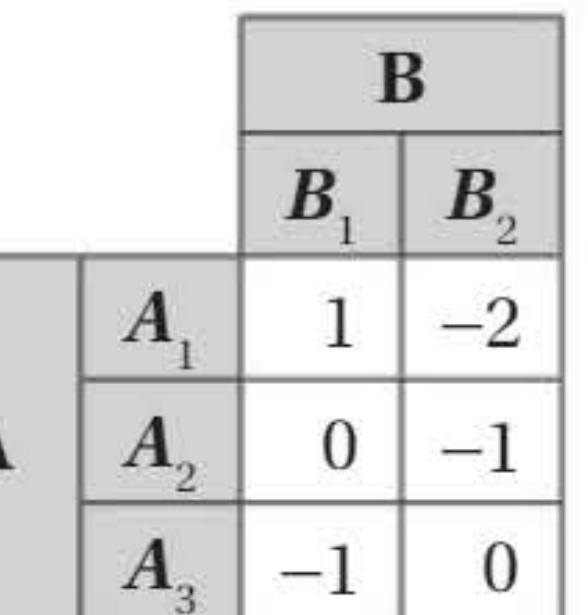
Worked example 3: using dominance
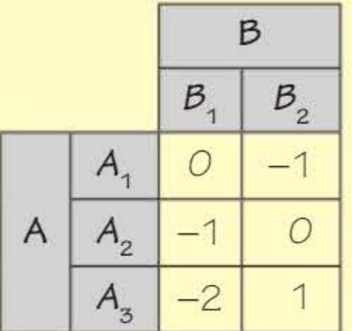
Worked Example: Reducing the Game Using Dominance
Problem: Show that this zero-sum game requires a mixed strategy, and find A's best strategy and the value of the game.
Solution:
Step 1: Use dominance to reduce the table
Column 2 dominates column 3 because every entry in column 2 is better for B (worse for A) than column 3:
- For A₁: (equal)
- For A₂: (B prefers column 2)
- For A₃: (B prefers column 2)
Since , , and , column 2 dominates column 3, so delete column 3.
The revised table is:
| B | |||
|---|---|---|---|
| B₁ | B₂ | ||
| A₁ | 0 | -1 | |
| A | A₂ | -1 | 0 |
| A₃ | -2 | 1 |
Step 2: Check for stable solution
Row minima: with maximum
Column maxima: with minimum
These are not equal, so the solution is not stable. We need a mixed strategy.
Step 3: Make all entries non-negative
Add 2 to all payoffs:
Step 4: Set up the linear programming problem
Suppose A plays A₁, A₂, and A₃ with probabilities , , and .
If B plays B₁, A's expected pay-off is:
If B plays B₂, A's expected pay-off is:
Maximise:
Subject to:
Step 5: Apply simplex algorithm
After introducing slack variables and applying the simplex method, the solution is:
So the value of the original game is
The optimal strategy for A is to play A₂ and A₃ with probabilities 0.75 and 0.25 respectively.
Key Insight on Dominance
Dominance allows us to simplify games before solving them:
- A row dominates another if all its entries are better (higher) for player A
- A column dominates another if all its entries are better (lower) for player B
- Always check for dominance first - it can significantly reduce problem complexity!
Strategy guide for solving zero-sum games
Follow these steps to solve any zero-sum game using linear programming:
- Construct a pay-off matrix (if necessary)
- Use dominance to reduce the table (if possible)
- A row dominates another if all its entries are better for A
- A column dominates another if all its entries are worse for A
- Check for a stable solution
- Calculate row minima and find their maximum
- Calculate column maxima and find their minimum
- If these are equal, the game has a pure strategy solution
- Write the problem as a linear programming formulation
- Define probability variables for each strategy
- Set objective: Maximise
- Write constraints for each opponent strategy
- Include probability constraint:
- Include non-negativity constraints
- Express constraints as equations using slack variables
- Convert all inequalities to equations
- Add slack variables where needed
- Apply the simplex algorithm
- Create initial tableau
- Perform row operations until objective row has no negative coefficients
- Read off the optimal probabilities and game value
- Values in final tableau give optimal mixed strategies
- Value is found in the final tableau
- Answer the question in context
- Remember to subtract any constant added to make entries non-negative
- Interpret results for both players
- State strategies clearly with their probabilities
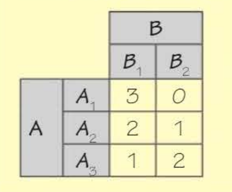
Worked example 4: 3×3 game without dominance
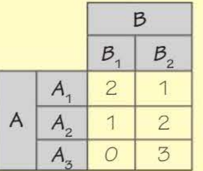
Worked Example: Solving a 3×3 Game Without Using Dominance
Problem: Solve this zero-sum game to find the optimal strategy for player A and the value of the game.
Solution:
The game cannot be reduced using dominance.
Step 1: Add 1 to all entries to make them non-negative:
| B | ||||
|---|---|---|---|---|
| B₁ | B₂ | B₃ | ||
| A₁ | 2 | 0 | 1 | |
| A | A₂ | 1 | 3 | 2 |
| A₃ | 2 | 2 | 0 |
Step 2: Suppose A plays A₁, A₂, and A₃ with probabilities , , and .
The linear programming formulation is:
Maximise:
Subject to:
Step 3: Introduce slack variables:
Step 4: After applying the simplex algorithm (which involves many row operations), the final solution is:
Therefore, the value of the original game is
The optimal strategy for A is to play A₁ and A₂ each with probability 0.5 (never play A₃).
Remember!
Key Points to Remember:
-
Zero-sum games involve two players where one's gain equals the other's loss, represented in a pay-off matrix showing outcomes for the row player.
-
A game has a stable solution (pure strategy) when the maximum of row minima equals the minimum of column maxima. Otherwise, use mixed strategies with probability distributions.
-
Expected pay-off for mixed strategies: where probabilities sum to 1.
-
To solve using linear programming:
- Add a constant to make all entries non-negative
- Formulate as maximising subject to constraints
- Introduce slack variables
- Apply the simplex algorithm
- Subtract the constant from the final value
-
8-Step Strategy Guide:
- Construct matrix
- Use dominance
- Check stability
- Write LP formulation
- Add slack variables
- Apply simplex
- Read solution
- Interpret results