Simplex Algorithm Revision Notes for AQA A-Level Further Maths

Simplex Algorithm

What is the simplex algorithm?

The simplex algorithm is an algebraic method used to solve linear programming problems. It systematically tests whether a vertex of the feasible region gives the optimal solution. If not, it moves to a better vertex and repeats the process until the optimal solution is found.

Linear programming involves finding the best combination of decision variables to maximise or minimise an objective function, subject to a set of constraints (usually inequalities). When you have only two decision variables, you can solve problems graphically by identifying the feasible region and using an objective line. However, when there are three or more decision variables, a graphical approach becomes difficult or impossible. This is where the simplex algorithm becomes essential.

infoNote

The simplex algorithm is particularly powerful because it:

Works efficiently with any number of decision variables
Guarantees finding the optimal solution (if one exists)
Systematically improves the solution at each step
Avoids testing every possible vertex of the feasible region

The simplex algorithm works by:

Converting the problem into a standard mathematical form
Creating a structured table (simplex tableau) to organize information
Performing systematic calculations to move from one solution to another
Testing for optimality at each step
Continuing until no better solution can be found

Slack variables and standard form

Slack variables

Before you can use the simplex algorithm, you must convert all inequality constraints into equations. This is done by introducing slack variables.

Definition: A slack variable represents the difference (the slack) between the two sides of an inequality constraint.

For example, if you have the constraint $4x + 3y \leq 1500$ , you introduce a slack variable $s$ to write:

$4x + 3y + s = 1500$

The slack variable $s \geq 0$ represents the unused capacity in this constraint. Similarly, for the constraint $x + 2y \leq 500$ , you introduce another slack variable $t$ :

$x + 2y + t = 500$

Consider the graphical representation of a linear programming problem:

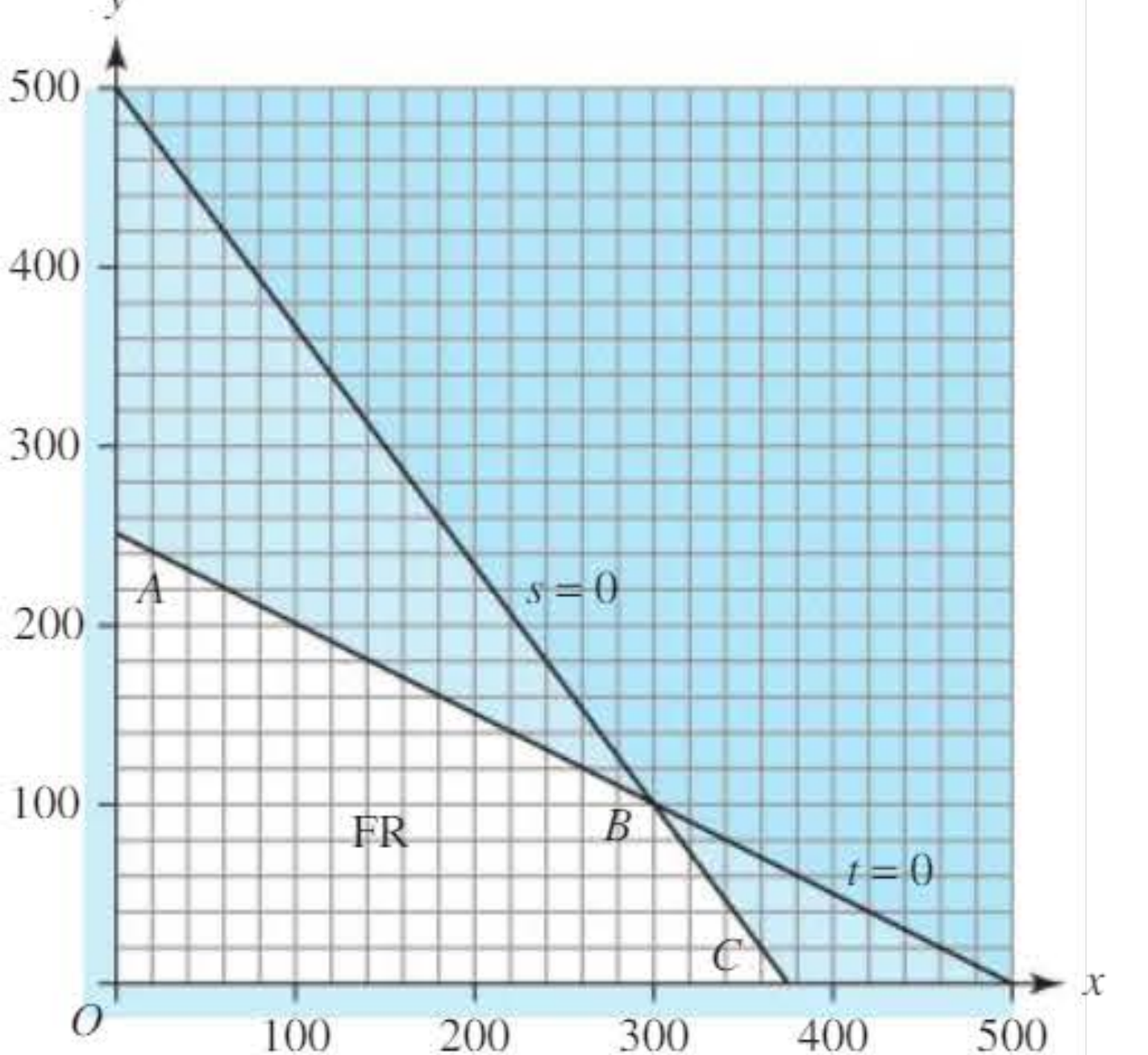
In this graph, the lines $s = 0$ and $t = 0$ represent the boundaries where the constraints are active (no slack). At each vertex of the feasible region, two of the variables are zero.

chatImportant

Key Insight About Slack Variables:

Each slack variable must be non-negative ( $s \geq 0, t \geq 0$ , etc.). When a slack variable equals zero, the constraint is "active" or "binding" - meaning you're using all available capacity. When the slack variable is positive, there's unused capacity in that constraint.

Standard form

To use the simplex algorithm, you must write your problem in standard form.

Standard form requirements:

All constraints must be written as equations (using slack variables)
All variables should appear on the left-hand side
A non-negative value should appear on the right-hand side
The objective function is also written in standard form (though the right-hand side can be negative)

lightbulbExample

Example: Converting to Standard Form

For the problem:

Maximise $P = 6x + 8y$

subject to:

$4x + 3y \leq 1500$
$x + 2y \leq 500$
$x \geq 0, y \geq 0$

Step 1: Introduce slack variables $s$ and $t$ for each constraint

Step 2: Write constraints as equations:

$4x + 3y + s = 1500$
$x + 2y + t = 500$

Step 3: Write objective in standard form:

$P - 6x - 8y - 0s - 0t = 0$

Complete standard form:

Maximise $P = 6x + 8y$

subject to:

$4x + 3y + s = 1500$
$x + 2y + t = 500$
$x \geq 0, y \geq 0, s \geq 0, t \geq 0$

This format makes it easier to enter the data into a simplex tableau.

The simplex tableau

Once your problem is in standard form, you organize the coefficients into a structured table called a simplex tableau (plural: tableaux).

Definition: A simplex tableau is a table that displays all the coefficients of the variables in your linear programming problem, organized in a way that facilitates the simplex algorithm calculations.

Structure of the initial tableau

The initial simplex tableau has:

A row for the objective function
A row for each constraint
Columns for each variable (decision variables and slack variables)
A 'Value' column showing the right-hand side values
A 'Row' column for recording operations (optional but helpful)
A 'Basic variable' column showing which variables form the current basis

Key features of the tableau:

The first row contains the objective function coefficients
Subsequent rows contain constraint coefficients
The 'Value' column shows the current values of basic variables
Basic variables have a coefficient of 1 in their row and 0 in all other rows

infoNote

Reading the Tableau:

Each row (except the objective row) represents one basic variable. The 'Value' column tells you the current value of that basic variable. The objective row's 'Value' entry shows the current value of the objective function.

Basic and non-basic variables

Understanding the concept of basic and non-basic variables is crucial for the simplex algorithm.

Definition: Basic variables are the variables that form the basis of the current solution. They have non-zero values and appear with a coefficient of 1 in exactly one row of the tableau, and 0 in all other rows.

Definition: Non-basic variables are set to zero in the current solution.

Basic solutions and basic feasible solutions

Each row in the tableau (except the objective row) represents a basic variable. At any stage of the algorithm:

The slack variables typically start as basic variables
Decision variables typically start as non-basic variables (set to zero)
As the algorithm progresses, variables change from non-basic to basic and vice versa

The initial tableau corresponds to the origin of the feasible region, where all decision variables are zero and the slack variables take their maximum values.

lightbulbExample

Example: Interpreting Basic and Non-Basic Variables

At the origin ( $x = 0, y = 0$ ):

Basic variables: $s = 1500$ , $t = 500$ (non-zero, using full slack)
Non-basic variables: $x = 0$ , $y = 0$ (set to zero)
Objective function value: $P = 0$

This represents the starting point where no production has occurred yet.

A basic feasible solution is a basic solution that also satisfies all constraints (all variables are non-negative). The vertices of the feasible region correspond to basic feasible solutions.

Here's a table showing all vertices:

chatImportant

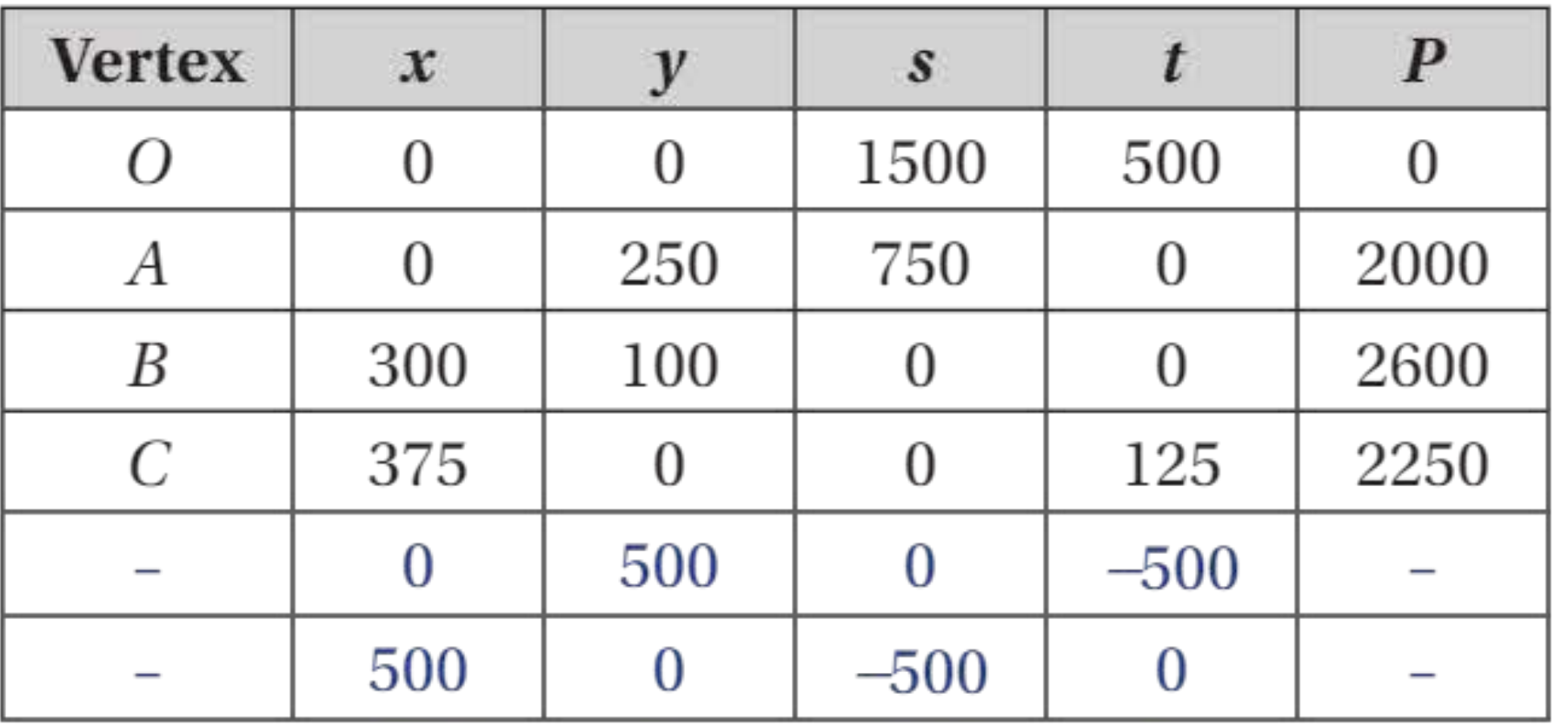
Feasibility Check:

The last two rows in this table have negative values for slack variables, which means they are not feasible solutions (not vertices of the feasible region). Remember: all variables must be non-negative for a solution to be feasible.

The simplex algorithm: step-by-step procedure

The simplex algorithm follows a systematic seven-step procedure to find the optimal solution.

Step 1: Write in standard form with slack variables

Express all constraints and the objective function as equations using slack variables. Ensure all right-hand side values are non-negative.

Step 2: Transfer data to a simplex tableau

Create the initial simplex tableau with the slack variables as the basic variables.

Step 3: Choose the pivot column

Key rule: Select the variable with the most negative coefficient in the objective row to enter the basis. This column is called the pivot column.

The most negative coefficient indicates which variable will increase the objective function most rapidly. In a maximisation problem, increasing this variable will improve the solution.

lightbulbExample

Example: Selecting the Pivot Column

If the objective row shows:

P	x	y	s	t
1	-6	-8	0	0

The $y$ -column has the most negative coefficient (-8), so it becomes the pivot column.

Interpretation: Increasing $y$ will increase $P$ by 8 units for each unit increase in $y$ (the largest rate of improvement).

Step 4: Calculate θ-values

For each positive entry in the pivot column, calculate the θ-value using:

$\theta_i = \frac{v_i}{p_i}$

where:

$v_i$ is the value in the 'Value' column for row $i$
$p_i$ is the entry in the pivot column for row $i$

chatImportant

Critical Rule for θ-values:

Only calculate θ-values for positive entries in the pivot column. Ignore zero or negative entries.

The θ-value represents how much the entering variable can increase before the basic variable in that row becomes zero (reaches its constraint limit).

Step 5: Choose the pivot row

Key rule: The row with the smallest θ-value is the pivot row. If there is a tie, choose any of the tied rows at random.

The smallest θ-value indicates which constraint will become active (reach its limit) first as you increase the entering variable.

Step 6: Identify the pivot

The entry at the intersection of the pivot column and pivot row is called the pivot or pivot element.

Step 7: Perform row operations

Now perform row operations to:

Divide the pivot row by the pivot element to make the pivot equal to 1
Use row operations on all other rows to create zeros elsewhere in the pivot column

The basic variable in the pivot row leaves the basis (becomes zero), and the variable for the pivot column enters the basis (becomes non-zero).

chatImportant

Working with Fractions:

Always use fractions, not decimals, to avoid rounding errors. Rounding can accumulate through multiple iterations and lead to incorrect final answers.

Step 8: Test for optimality

Optimality test: The solution is optimal when the objective row contains no negative coefficients.

If there are still negative coefficients in the objective row, return to Step 3 and repeat the process.

infoNote

Why This Test Works:

A negative coefficient in the objective row means that increasing that variable would increase the objective function. If no negative coefficients exist, no variable can improve the solution further - you've found the optimum!

Worked example 1: Two-variable problem

Let's solve the following problem using the simplex algorithm:

Maximise $P = 6x + 8y$

subject to:

$4x + 3y \leq 1500$
$x + 2y \leq 500$
$x \geq 0, y \geq 0$

lightbulbExample

Worked Example: Complete Simplex Solution

Step 1: Write in standard form with slack variables $s$ and $t$ :

$P - 6x - 8y - 0s - 0t = 0$ $4x + 3y + s + 0t = 1500$ $x + 2y + 0s + t = 500$

Step 2: Create the initial simplex tableau:

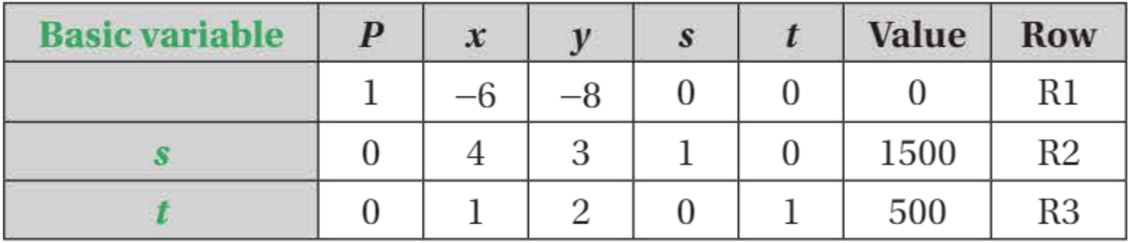
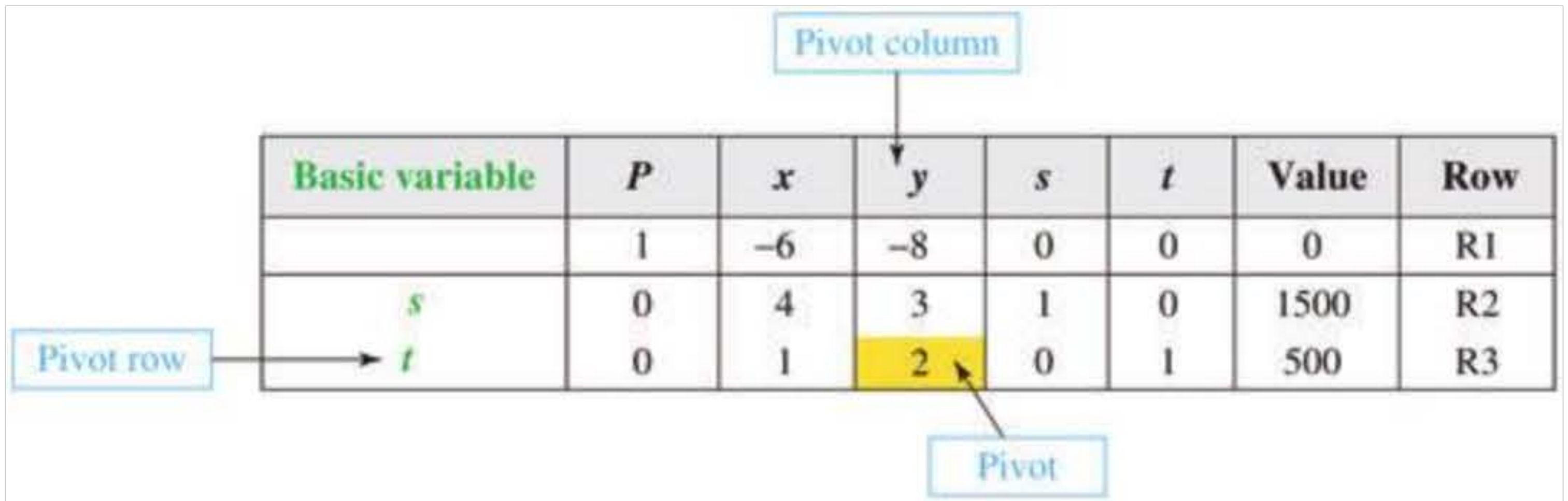
Basic variable	P	x	y	s	t	Value	Row
	1	-6	-8	0	0	0	R1
s	0	4	3	1	0	1500	R2
t	0	1	2	0	1	500	R3

At this stage: $x = 0, y = 0, s = 1500, t = 500, P = 0$

Step 3: The $y$ -column has the most negative coefficient (-8), so this is the pivot column.

Step 4: Calculate θ-values:

For row R2: $\theta = \frac{1500}{3} = 500$
For row R3: $\theta = \frac{500}{2} = 250$

Step 5: R3 has the smallest θ-value (250), so this is the pivot row. The pivot element is 2.

Step 6: Perform row operations. Divide R3 by 2 to get R6:

$R6 = \frac{R3}{2}$

Then:

$R4 = R1 + 8 \times R6$ (to eliminate $y$ from the objective row)
$R5 = R2 - 3 \times R6$ (to eliminate $y$ from the second constraint)

New tableau:

Basic variable	P	x	y	s	t	Value	Row
	1	-2	0	0	4	2000	R4
s	0	$2\frac{1}{2}$	0	1	$-1\frac{1}{2}$	750	R5
y	0	$\frac{1}{2}$	1	0	$\frac{1}{2}$	250	R6

At this stage: $x = 0, y = 250, s = 750, t = 0, P = 2000$

Step 7: Check for optimality. There is still a negative coefficient (-2) in the objective row, so we continue.

Iteration 2:

Step 3: The $x$ -column is now the pivot column (coefficient = -2).

Step 4: Calculate θ-values:

For R5: $\theta = \frac{750}{2\frac{1}{2}} = 300$
For R6: $\theta = \frac{250}{\frac{1}{2}} = 500$

Step 5: R5 has the smallest θ-value (300), so this is the pivot row. The pivot element is $2\frac{1}{2}$ .

Step 6: Divide R5 by $2\frac{1}{2}$ to get R8:

$R8 = \frac{R5}{2\frac{1}{2}}$

Then:

$R7 = R4 + 2 \times R8$
$R9 = R6 - \frac{1}{2} \times R8$

Final tableau:

Table

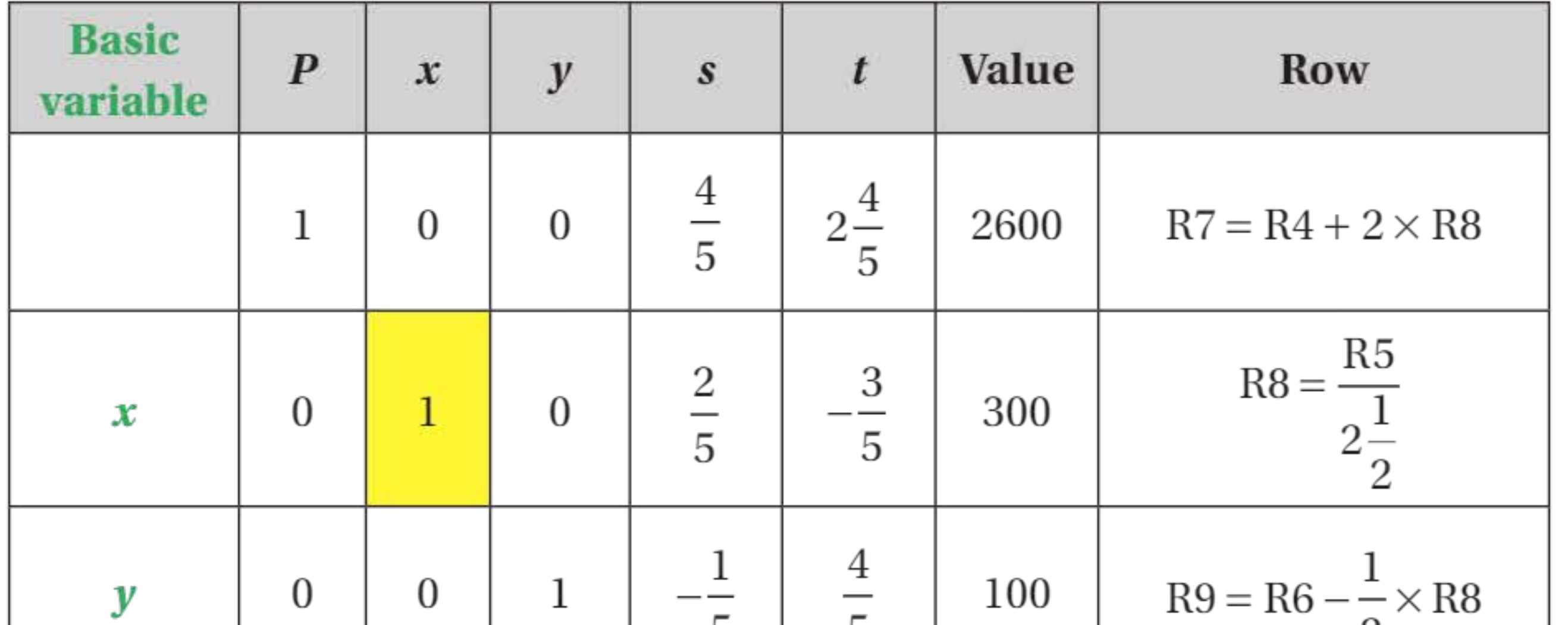
Basic variable	P	x	y	s	t	Value	Row
	1	0	0	$\frac{4}{5}$	$2\frac{4}{5}$	2600	R7
x	0	1	0	$\frac{2}{5}$	$-\frac{3}{5}$	300	R8
y	0	0	1	$-\frac{1}{5}$	$\frac{4}{5}$	100	R9

Step 7: There are no negative coefficients in the objective row, so the solution is optimal.

Final answer: $x = 300, y = 100, P = 2600$

The optimal solution is to set $x = 300$ and $y = 100$ , giving a maximum value of $P = 2600$ .

Worked example 2: Three-variable problem

Maximise $P = x + 2y + z$

subject to:

$x + 3y + 2z \leq 60$
$2x + y \leq 40$
$x + 3z \leq 30$
$x, y, z \geq 0$

lightbulbExample

Worked Example: Three-Variable Problem

Step 1: Introduce slack variables $s$ , $t$ , and $u$ :

$P - x - 2y - z = 0$ $x + 3y + 2z + s = 60$ $2x + y + t = 40$ $x + 3z + u = 30$

Step 2: Initial simplex tableau:

B.V.	P	x	y	z	s	t	u	Value	Row
	1	-1	-2	-1	0	0	0	0	R1
s	0	1	3	2	1	0	0	60	R2
t	0	2	1	0	0	1	0	40	R3
u	0	1	0	3	0	0	1	30	R4

Step 3: The $y$ -column has the most negative coefficient (-2), so this is the pivot column.

Step 4: Calculate θ-values:

R2: $\theta = \frac{60}{3} = 20$
R3: $\theta = \frac{40}{1} = 40$
R4: No positive entry (entry is 0)

Step 5: R2 is the pivot row (smallest θ-value of 20). The pivot is 3.

Step 6: Divide R2 by 3:

$R6 = \frac{R2}{3}$

Then perform row operations:

$R5 = R1 + 2 \times R6$
$R7 = R3 - R6$
$R8 = R4$ (unchanged as the entry is 0)

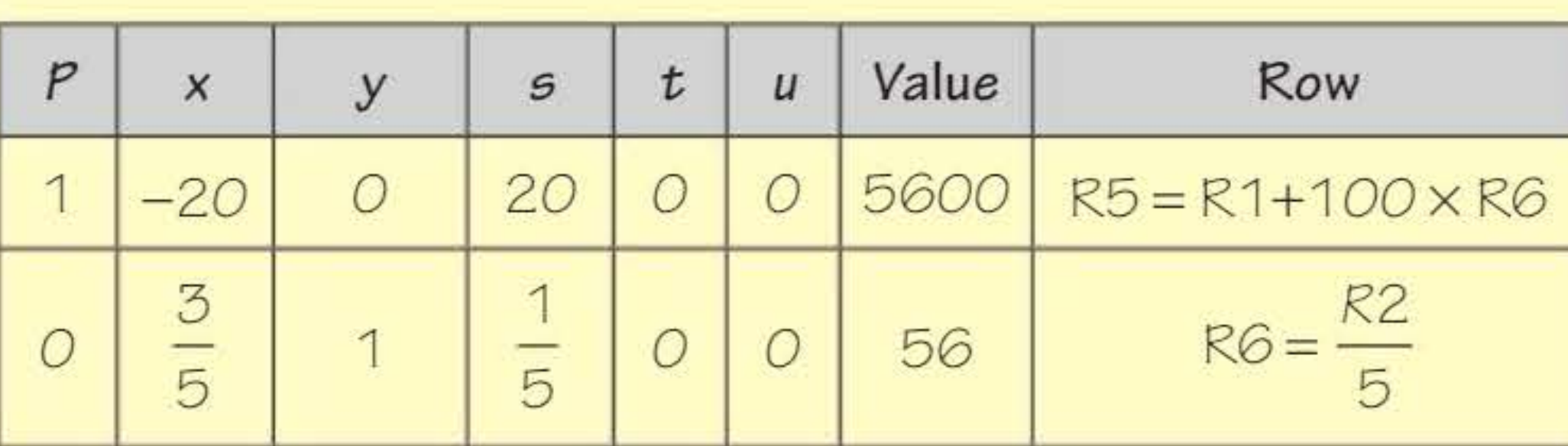
New tableau:

B.V.	P	x	y	z	s	t	u	Value	Row
	1	$-\frac{1}{3}$	0	$\frac{1}{3}$	$\frac{2}{3}$	0	0	40	R5
y	0	$\frac{1}{3}$	1	$\frac{2}{3}$	$\frac{1}{3}$	0	0	20	R6
t	0	$\frac{5}{3}$	0	$-\frac{2}{3}$	$-\frac{1}{3}$	1	0	20	R7
u	0	1	0	3	0	0	1	30	R8

There is still a negative coefficient in the objective row, so continue.

Iteration 2:

Step 3: The $x$ -column is the pivot column.

Step 4: Calculate θ-values:

R6: $\theta = \frac{20}{\frac{1}{3}} = 60$
R7: $\theta = \frac{20}{\frac{5}{3}} = 12$
R8: $\theta = \frac{30}{1} = 30$

Step 5: R7 is the pivot row (smallest θ = 12). The pivot is $\frac{5}{3}$ .

Step 6: Continue with row operations following the same pattern...

After completing the algorithm:

Final answer: $y = 16, x = 12, u = 18, P = 44$

The optimal solution is $x = 12$ , $y = 16$ , $z = 0$ , giving maximum $P = 44$ .

Note that $z = 0$ (non-basic), meaning this variable doesn't appear in the optimal solution.

Worked example 3: Minimisation problem

When you need to minimise an objective function, you can convert it to a maximisation problem.

chatImportant

Key Conversion Rule for Minimisation:

Minimising the objective function $C$ is equivalent to maximising the objective function $P = -C$ .

After finding the maximum value of $P$ , remember to convert back: $C = -P$

lightbulbExample

Worked Example: Minimisation Problem

Minimise $C = 3x - 4y - 3z$

subject to:

$x + y - z \geq -2$
$x + 2y + z \leq 3$
$x \geq 0, y \geq 0, z \geq 0$

Solution:

Step 1: Convert to maximisation:

Maximise $P = -3x + 4y + 3z$

Step 2: Rewrite the constraint $x + y - z \geq -2$ as an equation:

$-x - y + z + s = 2$

(We multiply by -1 to ensure the right-hand side is positive)

Step 3: Continue with standard form:

$x + 2y + z + t = 3$

Step 4: Create and solve the simplex tableau as normal.

After applying the simplex algorithm through multiple iterations, the final solution shows:

Final answer: Maximum $P = 8\frac{1}{3}$ when $x = 0$ , $y = \frac{1}{3}$ , $z = 2\frac{1}{3}$

Step 5: Convert back to minimisation:

Since $C = -P$ , the minimum value is:

$C = -8\frac{1}{3} = -8\frac{1}{3}$

when $x = 0$ , $y = \frac{1}{3}$ , $z = 2\frac{1}{3}$

Worked example 4: Non-standard constraints

Sometimes you encounter constraints that don't fit the standard form, such as $x + y \geq 2$ .

The simplex method requires the origin $(0, 0)$ to be a vertex of the feasible region. However, the constraint $x + y \geq 2$ means the origin is not in the feasible region.

infoNote

Handling Non-Standard Constraints:

To handle constraints with $\geq$ , you need to find an initial basic feasible solution before starting the simplex algorithm. One method is to pivot on a negative coefficient in the 'Value' column to eliminate the negative value and create a feasible starting point.

lightbulbExample

Worked Example: Non-Standard Constraints

Maximise $P = x + 2y$

subject to:

$2x + y \leq 6$
$x + y \geq 2$
$x, y \geq 0$

Solution:

Step 1: Rewrite the second constraint as $-x - y + t = -2$ (multiply by -1 and add slack variable)

The initial tableau would be:

P	x	y	s	t	Value	Row
1	-1	-2	0	0	0	R1
0	2	1	1	0	6	R2
0	-1	-1	0	1	-2	R3

The last constraint is not in standard form because the value is negative.

Step 2: Before starting the simplex algorithm, pivot on the cell shown to produce a +2 in the value column. Choose the pivot in R3 (the row with the negative value).

After pivoting to get a feasible starting solution:

P	x	y	s	t	Value	Row
1	0	-1	0	-1	2	R4
0	0	-1	1	2	2	R5
0	1	1	0	-1	2	R6

Step 3: Now apply the simplex algorithm with the pivot shown...

Final answer: Maximum $P = 12$ when $x = 0$ , $y = 6$ (with $t = 4$ )

Summary of the simplex algorithm

The complete simplex algorithm procedure:

bookmarkSummary

Step-by-Step Simplex Algorithm:

Step 1: Write the constraints and the objective function as equations in standard form, using slack variables.

Step 2: Transfer the data to a simplex tableau. At this stage the slack variables form the basis.

Step 3: Choose the column with the most negative coefficient in the objective row. This is the pivot column.

Step 4: If the positive numbers in the pivot column are $p_1, p_2, \ldots$ and the corresponding numbers in the 'Value' column are $v_1, v_2, \ldots$ , calculate:

$\theta_1 = \frac{v_1}{p_1}, \quad \theta_2 = \frac{v_2}{p_2}, \quad \ldots$

The row giving the smallest θ-value is the pivot row. (If there is a tie, choose at random). The number in the pivot column and pivot row is the pivot.

Step 5: Divide the pivot row by the pivot. Replace the basic variable for that row by the variable for the pivot column.

Step 6: Combine suitable multiples of the new pivot row with the other rows to give zeros in the pivot column.

Step 7: If there are no negative coefficients in the objective row, the solution is optimal. Otherwise, go to Step 3.

Conditions for using the standard simplex algorithm

You can use the standard simplex algorithm when:

You need to maximise the objective function
Every non-trivial constraint is an inequality using $\leq$
All variables are $\geq 0$
The origin is a vertex of the feasible region

chatImportant

When Standard Form Applies:

If these conditions are met, you can write the problem as equations in standard form using slack variables, with all right-hand sides being non-negative (except perhaps for the objective function).

If any condition is not met, you'll need to use modifications such as:

Converting minimisation to maximisation
Multiplying constraints by -1 to make right-hand sides positive
Finding an initial feasible solution before starting the algorithm

Real-world application example

A farmer has 65 hectares of land to grow wheat and potatoes. The costs and profits are shown in this table:

	Labour (man-hours per ha)	Fertiliser (kg per ha)	Profit (\£ per ha)
Wheat	30	700	80
Potatoes	50	400	100

There are 2800 man-hours of labour and 40 tonnes (40,000 kg) of fertiliser available.

lightbulbExample

Worked Example: Agricultural Planning Problem

Let $x$ = hectares of wheat and $y$ = hectares of potatoes.

Formulation:

Maximise $P = 80x + 100y$

subject to:

$30x + 50y \leq 2800$ (labour constraint)
$700x + 400y \leq 40000$ (fertiliser constraint)
$x + y \leq 65$ (land constraint)
$x \geq 0, y \geq 0$

After applying the simplex algorithm through multiple iterations:

Table

Final solution: Maximum profit = \£6050

Achieved by planting:

22.5 ha of wheat
42.5 ha of potatoes

The other non-zero value is $t = 72.5$ , which corresponds to 7250 kg of fertiliser left over.

This means the fertiliser constraint is not binding - the farmer has excess fertiliser available after the optimal allocation.

Key takeaways

bookmarkSummary

Remember These Key Points:

The simplex algorithm is used when you have three or more decision variables in a linear programming problem.
Slack variables convert inequality constraints into equations. They represent unused capacity in each constraint.
The solution is optimal when the objective row contains no negative coefficients.
Always choose the most negative coefficient in the objective row to select the pivot column.
Calculate θ-values for positive entries only: $\theta_i = \frac{v_i}{p_i}$ . The smallest θ-value determines the pivot row.
Use fractions, not decimals in calculations to avoid rounding errors.
To minimise an objective function $C$ , maximise $P = -C$ instead.
For non-standard problems (constraints with $\geq$ or minimisation), convert the problem into standard form before applying the simplex algorithm.

Mnemonics to Remember:

"No Negatives = Optimal"
"Most Negative Picks Pivot"
"Smallest Theta Selects Row"

Simplex Algorithm (AQA A-Level Further Maths): Revision Notes