Numerical Integration Revision Notes for AQA A-Level Further Maths

Numerical Integration

Introduction to numerical integration

When finding the area under a curve, we normally integrate the function between appropriate limits. However, some functions cannot be integrated using standard analytical methods. Examples include:

$y = \cos\left(\frac{1}{x}\right)$
$y = e^{x^2}$
$y = e^{\frac{1}{x}}$

Additionally, we may have experimental data from measurements where no equation for the curve exists. In these situations, we use numerical integration methods to estimate the area under the curve.

infoNote

Numerical integration is essential in two key scenarios:

When functions are theoretically impossible to integrate using standard calculus techniques
When working with real-world data where we only have measured values rather than a continuous function

Even though certain functions cannot be integrated analytically, they can still be plotted on a graph, and the area beneath them exists. Numerical methods allow us to approximate this area to a high degree of accuracy.

Mid-ordinate rule

What is the mid-ordinate rule?

The mid-ordinate rule is a straightforward numerical method that approximates the area under a curve by dividing the region into vertical rectangular strips. The height of each rectangle is determined by the y-value (ordinate) at the centre of that strip's width.

How the mid-ordinate rule works

To apply this method:

Divide the required area into $n$ equal vertical strips
Calculate the width of each strip: $d = \frac{b-a}{n}$ where $[a,b]$ is the interval
Find the y-value at the midpoint of each strip
Multiply each y-value by the strip width
Sum all the rectangular areas

chatImportant

Key advantage of the mid-ordinate rule:

Errors tend to balance out. Where a small area above the curve is included (over-estimate), there is usually a corresponding small area beneath the curve that is missed (under-estimate). This compensation improves the overall accuracy.

Mid-ordinate rule formula

Definition: If we divide the area to be estimated under a function from $a$ to $b$ into $n$ rectangles, and let the ordinates at the centre of each rectangle be $y_1, y_2, \ldots, y_n$ , then the estimated area is:

$A = \frac{b-a}{n}(y_1 + y_2 + y_3 + \cdots + y_n)$

infoNote

Key point: The more rectangles used, the more accurate the estimate becomes, because each strip width decreases and the rectangles fit the curve more closely.

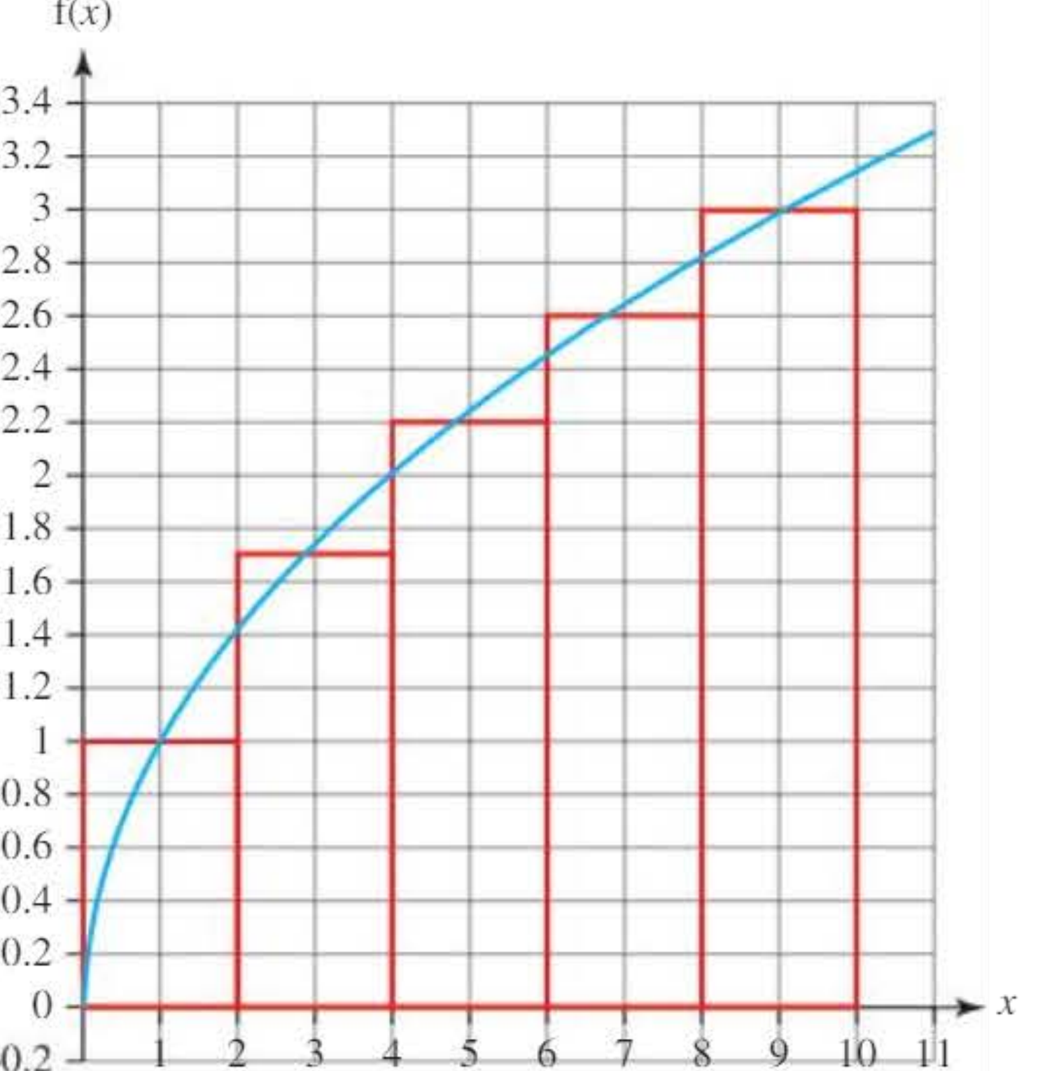
Worked example 1: Mid-ordinate rule with quadratic function

lightbulbExample

Worked Example: Applying the Mid-ordinate Rule

Problem: For the function $y = 10x - x^2$ :

Draw the graph
Divide the area between the curve and the x-axis into 10 rectangles
Estimate the area using the mid-ordinate rule
Find the exact area using calculus
Calculate the relative error

Solution:

Part (a): The graph shows a parabola opening downwards with maximum at $x = 5$ .

Part (b): With 10 rectangles from $x = 0$ to $x = 10$ , the width of each rectangle is: $d = \frac{10-0}{10} = 1$

Part (c): The mid-ordinates occur at $x = 0.5, 1.5, 2.5, 3.5, 4.5, 5.5, 6.5, 7.5, 8.5, 9.5$

Calculate each y-value:

At $x = 0.5$ : $y = 10(0.5) - (0.5)^2 = 4.75$
At $x = 1.5$ : $y = 10(1.5) - (1.5)^2 = 12.75$
At $x = 2.5$ : $y = 10(2.5) - (2.5)^2 = 18.75$

Continuing this pattern and summing:

A = 1 \times [(10 \times 0.5 - 0.5^2) + (10 \times 1.5 - 1.5^2) + \cdots + (10 \times 9.5 - 9.5^2)]

A = 1 \times [4.75 + 12.75 + 18.75 + 22.75 + 24.75 + 24.75 + 22.75 + 18.75 + 12.75 + 4.75]

A = 162.75

Part (d): Using integration to find the exact area:

$\int_0^{10} (10x - x^2)\,dx = \left[5x^2 - \frac{x^3}{3}\right]_0^{10}$

$= 5(10)^2 - \frac{(10)^3}{3} - 0 = 500 - \frac{1000}{3} = \frac{500}{3} = 166\frac{2}{3}$

Part (e): The relative error is calculated as:

$\text{Relative error} = \frac{\text{approximate} - \text{exact}}{\text{exact}} = \frac{162.75 - 166.67}{166.67} = -0.0235 \text{ (3 s.f.)}$

The negative value indicates the approximation underestimated the true area by approximately 2.35%.

Simpson's rule

Why Simpson's rule?

While the mid-ordinate rule is simple to apply, Thomas Simpson published a more sophisticated method in 1743 that achieves greater accuracy. Simpson's rule eliminates the discrepancies at the top of each rectangle by replacing the mid-ordinates with a quadratic curve (parabola). Just as you can always draw a straight line between two points, you can always draw a parabola through three points.

Understanding Simpson's rule

Simpson's rule works by fitting a parabola through three consecutive points on the curve. The area under this parabola can be calculated exactly using integration.

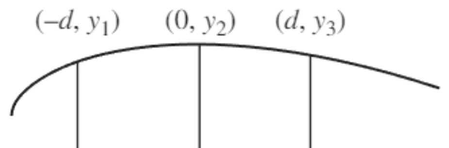
Consider three points on a parabola with equation $y = ax^2 + bx + c$ , positioned symmetrically at $(-d, y_1)$ , $(0, y_2)$ , and $(d, y_3)$ .

The area under this parabola from $-d$ to $d$ is:

$A = \int_{-d}^{d} (ax^2 + bx + c)\,dx = \left[\frac{ax^3}{3} + \frac{bx^2}{2} + cx\right]_{-d}^{d} = \frac{2}{3}ad^3 + 2cd$

By substituting the three coordinate points into the parabola equation, we can show that:

$y_1 = ad^2 - bd + c$
$y_2 = c$
$y_3 = ad^2 + bd + c$

Adding these equations: $y_1 + 4y_2 + y_3 = 2ad^2 + 6c$

Multiplying by $\frac{d}{3}$ :

$\frac{d}{3}(y_1 + 4y_2 + y_3) = \frac{2}{3}ad^3 + 2cd = A$

This is Simpson's rule for three points:

$A = \frac{d}{3}(y_1 + 4y_2 + y_3)$

Extension to multiple strips

To find the area under a longer section of curve, we divide it into an even number of strips, creating pairs of strips. Each pair uses Simpson's formula.

For example, with 8 strips (4 pairs), the total area is:

$A = \frac{d}{3}(y_0 + 4y_1 + y_2) + \frac{d}{3}(y_2 + 4y_3 + y_4) + \frac{d}{3}(y_4 + 4y_5 + y_6) + \frac{d}{3}(y_6 + 4y_7 + y_8)$

Collecting terms:

$A = \frac{d}{3}[(y_0 + y_8) + 4(y_1 + y_3 + y_5 + y_7) + 2(y_2 + y_4 + y_6)]$

General Simpson's rule formula

Definition: If the area required is divided into $n$ strips of equal width $d$ , where $n$ is even, then:

$\int_{x_0}^{x_n} f(x)\,dx = \frac{d}{3}\left[(y_0 + y_n) + 4(y_1 + y_3 + y_5 + \cdots + y_{n-1}) + 2(y_2 + y_4 + y_6 + \cdots + y_{n-2})\right]$

chatImportant

Critical requirement: Simpson's rule requires an even number of strips. This is non-negotiable for the method to work correctly.

Pattern of coefficients: 1-4-2-4-2-4-2-...-4-2-4-1

The pattern is:

First and last ordinates: coefficient of 1
Odd-numbered ordinates: coefficient of 4
Even-numbered ordinates (except first and last): coefficient of 2

infoNote

Simpson's rule is much more accurate than dividing the area into just two strips using the mid-ordinate rule, even when using fewer strips overall.

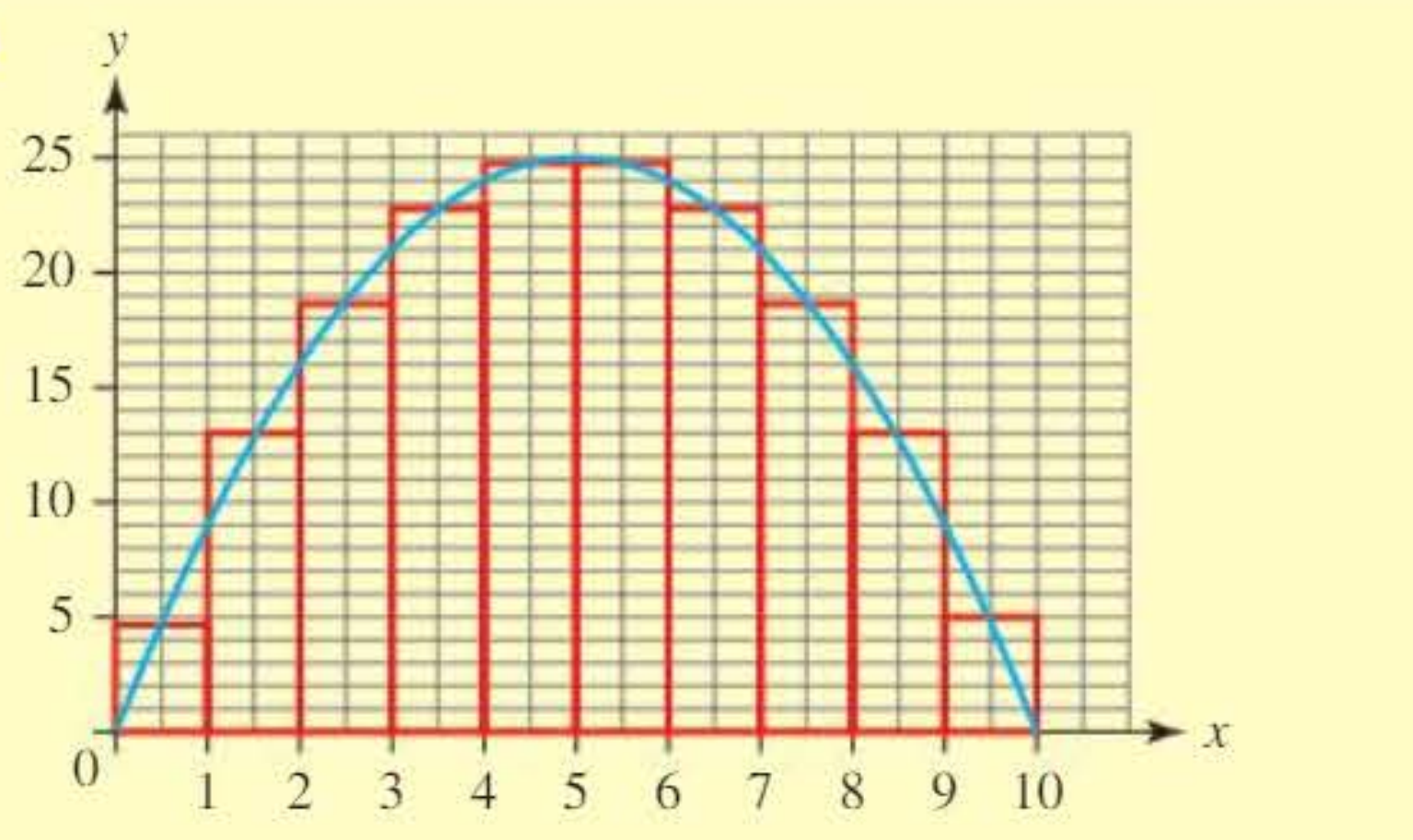
Worked example 2: Simpson's rule with quadratic function

lightbulbExample

Worked Example: Simpson's Rule with a Quadratic

Problem: Use Simpson's rule with ten strips to find the approximate area for $y = 10x - x^2$ from $x = 0$ to $x = 10$ .

Solution:

With $n = 10$ strips, the width is $d = 1$ .

Create a table of values:

$x$	0	1	2	3	4	5	6	7	8	9	10
$y$	0	9	16	21	24	25	24	21	16	9	0

Apply Simpson's formula:

$A = \frac{1}{3}[(0 + 0) + 4(9 + 21 + 25 + 21 + 9) + 2(16 + 24 + 24 + 16)]$

$= \frac{1}{3}[0 + 4(85) + 2(80)]$

$= \frac{1}{3}[340 + 160] = \frac{500}{3} = 166\frac{2}{3}$

Comment: Since $y = 10x - x^2$ is a quadratic function and Simpson's rule uses parabolic approximation, the answer is exact rather than approximate.

Worked example 3: Volume of a vase

lightbulbExample

Worked Example: Finding Volume Using Simpson's Rule

Problem: A decorative vase has circular cross-sections. The radius $r$ cm at height $h$ cm above the base is shown in the table below. The vase is 40 cm high. Estimate the volume in litres.

$h$	0	5	10	15	20	25	30	35	40
$r$	6	5	11	13	15	13	11	5	6

Solution:

The volume can be found by calculating the area under a graph of circular cross-sectional area ( $\pi r^2$ ) plotted against height.

With 8 strips, width $d = 5$ cm.

The areas of cross-sections are: $\pi \times 6^2, \pi \times 5^2, \pi \times 11^2$ , etc.

Using Simpson's rule:

$V = \frac{5}{3}[(\pi \times 6^2 + \pi \times 6^2) + 4(\pi \times 5^2 + \pi \times 13^2 + \pi \times 13^2 + \pi \times 5^2) + 2(\pi \times 11^2 + \pi \times 15^2 + \pi \times 11^2)]$

$= \frac{5\pi}{3}[(72) + 4(388) + 2(467)]$

$= \frac{5\pi}{3}[72 + 1552 + 934] = \frac{5\pi}{3}(2558)$

$= 13394 \text{ cm}^3 = 13.394 \text{ litres}$

Worked example 4: Estimating π

lightbulbExample

Worked Example: Estimating π Using Numerical Integration

Problem: The equation of a circle with radius 12 is $x^2 + y^2 = 144$ . Using Simpson's rule in the first quadrant with 12 equal intervals, find an estimate for $\pi$ correct to 2 decimal places. Calculate the relative error.

Solution:

From $x^2 + y^2 = 144$ , we get $y = \sqrt{144 - x^2}$

The area in the first quadrant is: $A = \int_0^{12} \sqrt{144 - x^2}\,dx$

With 12 strips, $d = 1$ . Calculate y-values:

$x$	0	1	2	3	4	5	6	7	8	9	10	11	12
$y$	12	11.958	11.832	11.619	11.314	10.909	10.392	9.747	8.944	7.937	6.633	4.796	0

Apply Simpson's rule:

$A = \frac{1}{3}[(12 + 0) + 4(11.958 + 11.619 + 10.909 + 9.747 + 7.937 + 4.796) + 2(11.832 + 11.314 + 10.392 + 8.944 + 6.633)]$

$= \frac{1}{3}[12 + 4(56.966) + 2(49.115)]$

$= \frac{1}{3}[12 + 227.864 + 98.23] = \frac{338.094}{3} = 112.698$

This area represents one quarter of the circle's area:

$\frac{1}{4} \times \pi \times 12^2 = 112.698$

$36\pi = 112.698$

$\pi = \frac{112.698}{36} = 3.13$

The relative error is:

$\text{Relative error} = \frac{3.13 - 3.14}{3.14} = -0.003$

The estimate is accurate to within 0.3%.

Accuracy and error calculation

Relative error formula

To assess how accurate an approximation is, we calculate the relative error:

$\text{Relative error} = \frac{\text{approximate value} - \text{exact value}}{\text{exact value}}$

This gives a proportional measure of the error. A negative relative error indicates the approximation is less than the exact value (underestimate), while a positive value indicates an overestimate.

Comparing methods

infoNote

Mid-ordinate rule:

Simple to apply
Reasonable accuracy with sufficient rectangles
Errors partially cancel due to over and under-estimation

Simpson's rule:

More accurate than mid-ordinate rule
Uses parabolic approximation
Requires even number of strips
Gives exact results for quadratic functions
Preferred for higher accuracy requirements

Exam tips

chatImportant

Common Pitfalls to Avoid:

Always check if n is even when using Simpson's rule
Show your working clearly, including the coefficient pattern (1-4-2-4-...-1)
Calculate relative error to 3 or 4 significant figures unless specified otherwise
Remember: more strips generally means better accuracy, but Simpson's rule with fewer strips often beats mid-ordinate rule with more strips
For quadratic functions, Simpson's rule gives the exact answer
When creating tables of values, work systematically and check your arithmetic

Remember!

bookmarkSummary

Key Points to Remember:

Numerical integration is used when functions cannot be integrated analytically or when working with experimental data only.
Mid-ordinate rule formula: $A = \frac{b-a}{n}(y_1 + y_2 + \cdots + y_n)$ where ordinates are taken at the centre of each strip. More rectangles improve accuracy.
Simpson's rule is more accurate because it uses parabolic curves instead of rectangles. The coefficient pattern is 1-4-2-4-2-...-4-2-4-1, and it requires an even number of strips.
Simpson's rule formula: $\int_{x_0}^{x_n} f(x)\,dx = \frac{d}{3}[(y_0 + y_n) + 4(\text{odd ordinates}) + 2(\text{even ordinates})]$ where $d$ is the strip width.
Relative error measures accuracy: $\frac{\text{approximate} - \text{exact}}{\text{exact}}$ . A negative value means underestimation; positive means overestimation.

Numerical Integration (AQA A-Level Further Maths): Revision Notes