Real operational amplifiers (AQA A-Level Physics): Revision Notes

13.4.4 Real operational amplifiers

Characteristic	Ideal Op-Amp	Real Op-Amp
Open-Loop Gain ($A_\text{OL}$)	Infinite	Around $10^6$
Input Resistance $(R_\text{in})$	Infinite, no current draw	Up to $10^{12} \, \Omega$
Output Resistance $(R_\text{out})$	Zero	Around $100 \, \Omega$
Output Voltage $(V_\text{out})$	Bounded between $\pm V_S$	Limited, and can vary slightly due to resistance
Bandwidth	Infinite (at any frequency)	Limited, around $15$ Hz (open-loop), and up to $2.5$ MHz (closed-loop)

Real op-amps are also affected by temperature, which can alter these values slightly.

Key Differences in Real Op-Amps

1. Open-Loop Gain $(A_\text{OL})$ While real op-amps have high open-loop gain, it is not infinite. This gain remains sufficient for most applications, but deviations may occur, especially under varying temperature conditions or high frequencies.

2. Input Resistance $(R_\text{in})$ Real op-amps have high input resistance, drawing very little current (on the scale of nanoamperes). This small current can impact sensitive measurements, but generally, high input resistance remains suitable for many applications.

3. Output Resistance $(R_\text{out})$ Real op-amps have a non-zero output resistance, limiting the current they can deliver. When negative feedback is used in a circuit, output resistance decreases, which stabilises the output but may restrict available current.

4. Offset Voltage In an ideal op-amp, when both inputs are grounded, the output should be zero. However, real op-amps have a small offset voltage (a slight non-zero output). To counter this, op-amps often include a mechanism for offset nulling to calibrate the device.

Frequency Response and Bandwidth

1. Bandwidth Limitations Real op-amps exhibit limited bandwidth in open-loop configurations due to their high gain. Most data sheets specify the closed-loop bandwidth, as unity gain configurations (also called unity gain buffers) allow for wider bandwidth but lower gain.

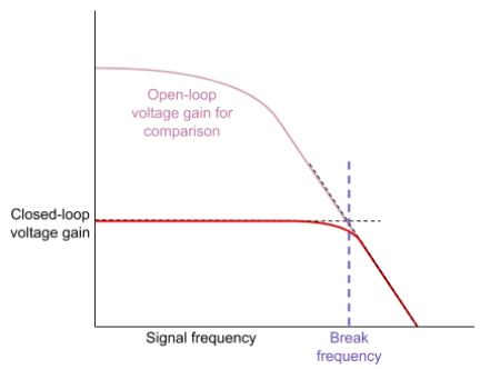
2. Frequency Response Curves Frequency response curves illustrate how the gain of an op-amp changes with signal frequency. Typically, these curves are logarithmic to accommodate high values of frequency and gain.

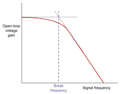
3. Break Frequency

• The break frequency is the point where the gain begins to drop. It is often determined by plotting straight-line approximations of the curve and locating their intersection.
• In open-loop configurations, the break frequency is low. However, closed-loop circuits have a much higher break frequency, making them preferable for high-frequency applications.

4. Gain-Bandwidth Product The gain-bandwidth product remains constant for a given op-amp, summarised by:

$$\text{gain} \times \text{bandwidth} = \text{constant}$$

This relationship means that increasing gain will reduce the available bandwidth and vice versa.