Quantitative Sales Forecasting Revision Notes for Edexcel A-Level Business

Quantitative sales forecasting

Introduction to quantitative sales forecasting

Quantitative sales forecasting uses statistical techniques to predict future sales based on historical data. This approach is essential for business planning, helping managers make informed decisions about production, staffing, inventory, and cash flow. Unlike qualitative methods that rely on opinions, quantitative forecasting provides numerical predictions based on mathematical analysis of past trends.

The main tool used in quantitative forecasting is time series analysis, which examines data collected over consecutive time periods (such as quarters or years) to identify patterns and trends. By understanding these patterns, businesses can project future performance with greater accuracy.

infoNote

The key advantage of quantitative forecasting over qualitative methods is its reliance on objective numerical data rather than subjective opinions. This makes predictions more defensible and easier to update as new data becomes available.

Components of time series data

Time series data contains four main components that businesses must identify:

Trend: The underlying long-term direction of the data, showing whether values are generally increasing, decreasing, or remaining stable over time.

Seasonal fluctuations: Regular variations that occur within a year, repeating in a predictable pattern (e.g., higher sales in summer for ice cream).

Cyclical fluctuations: Longer-term variations linked to economic cycles, typically lasting several years.

Random fluctuations: Unpredictable variations caused by unexpected events or factors.

chatImportant

This unit focuses primarily on identifying and using the trend component for forecasting purposes. While all four components exist in most time series data, the trend provides the foundation for making future predictions.

Calculating moving averages

Moving averages smooth out short-term fluctuations in data to reveal the underlying trend. The technique involves calculating the average of successive groups of values, creating a series of averages that "move" through the dataset.

Three-period moving average

To calculate a three-period moving average:

Add the first three consecutive values
Divide by 3 to find the average
Drop the first value and add the next value
Repeat the process

lightbulbExample

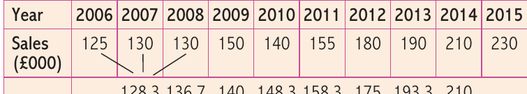
Worked Example: Three-Period Moving Average

For sales of 125, 130, and 130:

First moving average = $(125 + 130 + 130) \div 3 = 128.3$
Second moving average = $(130 + 130 + 150) \div 3 = 136.7$

The moving average is placed at the centre of the period used. For a three-year average calculated from 2006-2008, the result is placed next to 2007.

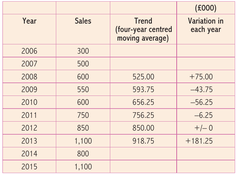
Four-period moving average and centring

When using an even number of periods (such as quarterly data), there is no natural centre point. The solution is centring, which uses both four-period and eight-period moving totals to find a mid-point.

The centring process:

Calculate four consecutive values and find their total (four-period moving total)
Calculate the next four consecutive values and find their total
Add these two four-period totals together (eight-period moving total)
Divide the eight-period total by 8 to find the centred moving average

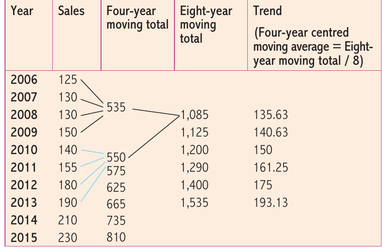
The formula for the trend is:

$\text{Four-period centred moving average} = \frac{\text{Eight-period moving total}}{8}$

infoNote

This technique ensures the moving average aligns properly with specific time periods, making it suitable for quarterly data analysis. Without centring, the results would fall between time periods rather than on them, making the data difficult to interpret and use for forecasting.

Plotting trends and identifying patterns

Once moving averages are calculated, plotting them on a graph reveals the trend clearly. The trend line appears smoother than the actual sales figures because it eliminates short-term fluctuations.

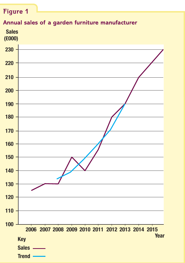
The graph shows:

Actual sales (darker line): Shows year-to-year variations
Trend (lighter line): Shows the underlying direction after smoothing

The trend line helps businesses understand whether their performance is improving, declining, or stable over time, independent of temporary variations.

Predicting future values using extrapolation

Extrapolation means extending past trends into the future to make predictions. This involves drawing a line of best fit through the trend data and extending it forward.

Drawing the line of best fit

The line of best fit is drawn so that:

It matches the general slope of the trend points
Points on one side of the line balance with points on the other side
It represents the average direction of all trend values

For greater accuracy, the line should pass through the coordinates $(\bar{X}, \bar{Y})$ where:

$\bar{X}$ = mean of the years
$\bar{Y}$ = mean of the sales values

lightbulbExample

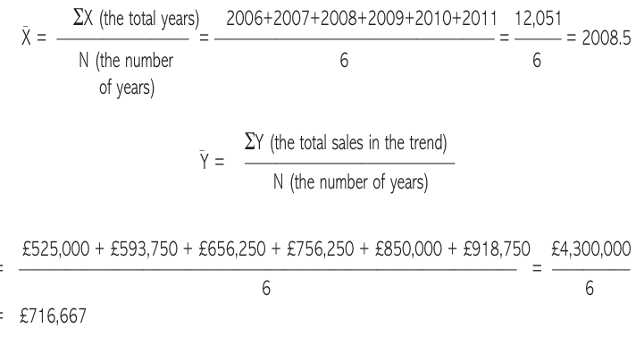
Worked Example: Calculating Mean Coordinates

Mean year:

$\bar{X} = \frac{2006 + 2007 + 2008 + 2009 + 2010 + 2011}{6} = \frac{12,051}{6} = 2008.5$

Mean sales:

$\bar{Y} = \frac{\text{\$525,000} + \text{\$593,750} + \text{\$656,250} + \text{\$756,250} + \text{\$850,000} + \text{\$918,750}}{6}$

$\bar{Y} = \frac{\text{\$4,300,000}}{6} = \text{\$716,667}$

By extending the line of best fit beyond the available data, businesses can estimate future sales. However, this assumes that no significant changes will occur to affect the existing trend.

chatImportant

Critical Assumption: Extrapolation assumes that the factors influencing past trends will continue unchanged into the future. This is often unrealistic, especially for longer-term forecasts where market conditions, competition, and customer preferences may change significantly.

Calculating variations from the trend

The trend smooths out fluctuations, but actual values vary around the trend line. To improve forecast accuracy, businesses calculate the variation between actual values and trend values.

Cyclical variation

Formula:

$\text{Variation} = \text{Actual sales} - \text{Trend}$

For each period with both actual sales and trend data, calculate the difference. Some variations will be positive (actual sales above trend) and some negative (actual sales below trend).

Average cyclical variation is calculated as:

$\text{Average cyclical variation} = \frac{\text{Sum of all variations}}{\text{Number of variations}}$

lightbulbExample

Worked Example: Applying Cyclical Variation

Add the average variation to the trend prediction to create a more accurate forecast:

Trend prediction for 2016 = $1,160,000
Average variation = +$25,000
Adjusted prediction = $1,185,000

Seasonal variation

Seasonal variations occur within a year, typically calculated for quarterly data. The same variation formula applies, but patterns emerge for specific quarters.

Process for seasonal forecasting:

Calculate the trend prediction for the target quarter
Find all variations for that specific quarter in previous years
Calculate the average seasonal variation for that quarter
Add (or subtract if negative) the average seasonal variation from the trend prediction

lightbulbExample

Worked Example: Seasonal Variation Adjustment

Step 1: Identify the trend prediction

Trend prediction for Q4 2015 = $470,000

Step 2: Calculate average Q4 variation

Average Q4 variation = $\frac{-\text{\$ 97,125} + (-\text{$117,500})}{2} = -\text{$107,313}$

Step 3: Apply the adjustment

Adjusted prediction = $470,000 − $107,313 = $362,687

infoNote

This approach accounts for the fact that certain quarters consistently perform above or below the general trend. For example, retail businesses typically experience higher sales in Q4 due to holiday shopping, while other quarters may be consistently lower.

Limitations of quantitative sales forecasts

Despite their mathematical basis, quantitative forecasts have significant limitations. Past performance does not guarantee future results, and several factors affect forecast reliability.

Forecasts are more reliable when:

Short time horizons: Predictions for six months ahead are more accurate than five-year forecasts, as fewer unexpected changes can occur.

Frequent updates: Regular revision using new data keeps forecasts current and relevant.

Stable markets: In slow-changing industries, past patterns are more likely to continue.

Market research available: Primary and secondary research data, including test marketing results, improves forecast accuracy.

Experienced forecasters: Those with good understanding of both statistical techniques and market dynamics produce better forecasts.

Qualitative input: Expert judgment and "feel" for the market can adjust forecasts to account for factors not captured in historical data.

Forecast ranges

Rather than a single prediction, sophisticated forecasts provide a range of outcomes:

Optimistic forecast: Best-case scenario with lower probability

Central forecast: Most likely outcome with highest probability

Pessimistic forecast: Worst-case scenario with lower probability

infoNote

This approach acknowledges uncertainty and helps other departments (such as production) prepare for different scenarios. By planning for a range of outcomes rather than a single prediction, businesses can respond more flexibly to actual market conditions.

Despite imperfections, quantitative forecasts remain valuable tools for planning and budgeting.

Correlation and causal modelling

While time series analysis describes trends over time, causal modelling attempts to explain data by finding relationships between different variables.

Scatter graphs and correlation

A scatter graph plots two variables to visualize their relationship:

Independent variable (X-axis): The factor believed to influence outcomes (e.g., advertising expenditure)
Dependent variable (Y-axis): The outcome being measured (e.g., sales)

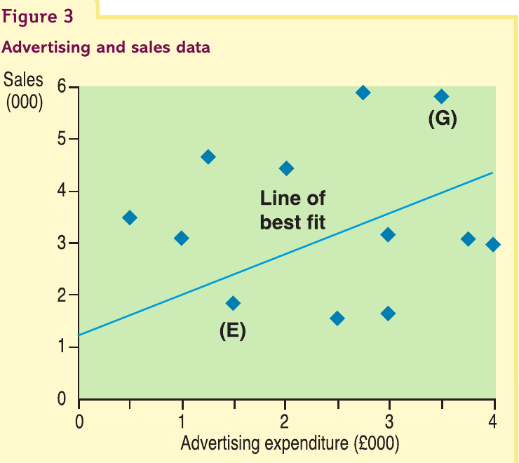
Each point represents data from a specific period, showing the combination of both variables at that time.

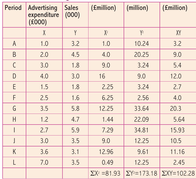
The correlation coefficient

The correlation coefficient $(r)$ measures the strength and direction of the relationship between two variables.

Formula:

$r = \frac{\sum XY}{\sqrt{(\sum X^2)(\sum Y^2)}}$

Where:

$\sum XY$ = sum of $(X \times Y)$ for all data points
$\sum X^2$ = sum of $X^2$ for all data points
$\sum Y^2$ = sum of $Y^2$ for all data points

Interpreting correlation coefficients:

$r = +1$ : Perfect positive correlation - all points fall exactly on an upward-sloping line. As X increases, Y increases proportionally.

$r = 0$ : No correlation - the variables are not related to each other.

$r = -1$ : Perfect negative correlation - all points fall exactly on a downward-sloping line. As X increases, Y decreases proportionally.

$r = +0.86$ (example): Strong positive correlation - most points cluster around an upward-sloping line, suggesting advertising increases lead to higher sales.

infoNote

Values below 0.7 (positive or negative) indicate weak correlations that are difficult to identify visually on scatter graphs. In business contexts, correlation coefficients between 0.7 and 1.0 (or -0.7 and -1.0) are considered strong enough to be meaningful.

Types of correlation

Positive correlation: Both variables move in the same direction (e.g., advertising spending and sales both increase).

Negative correlation: Variables move in opposite directions (e.g., as price increases, demand decreases).

No correlation: Variables show no clear relationship (e.g., quantity of baked beans sold and sofa sales).

Cautions with correlation

Other influencing factors: High sales might result from factors beyond advertising, such as competitor actions or economic conditions.

Nonsense correlations: Sometimes two variables show statistical correlation purely by coincidence, with no genuine causal relationship.

Correlation ≠ causation: Even strong correlation doesn't prove one variable causes changes in the other - both might be influenced by a third factor.

chatImportant

Critical Distinction: Correlation vs Causation

Just because two variables are correlated does not mean one causes the other. For example:

Ice cream sales and drowning incidents are correlated, but ice cream doesn't cause drowning
Both are influenced by a third factor: hot weather
Always look for logical causal mechanisms, not just statistical relationships

Businesses should use correlation analysis carefully, combining statistical findings with market knowledge and business judgment.

Qualitative forecasting

While this unit focuses on quantitative methods, qualitative forecasting plays an important complementary role. This approach uses expert opinions and experienced judgments rather than numerical data.

When qualitative forecasting is appropriate:

Insufficient numerical data: New products or markets lack historical data for quantitative analysis.

Rapidly changing markets: In dynamic industries, historical data becomes outdated quickly, making expert judgment more valuable.

Qualitative methods include expert panels, Delphi techniques, and management experience. Often, businesses combine quantitative forecasts with qualitative insights for more robust predictions.

Exam technique for quantitative forecasting

When answering exam questions on this topic:

Analysis opportunities:

Calculate moving averages and trends from provided data
Interpret what trends reveal about business performance
Use extrapolation to predict future values
Calculate and explain correlation coefficients

Evaluation considerations:

Question the reliability of predictions based on limited data
Consider external factors that might disrupt trends
Assess whether past patterns will continue
Recognize the limitations of the forecasting method used

The "it depends" principle:

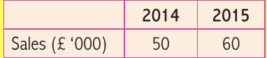
If sales grew from $50,000 to $60,000, will they continue growing?

It depends on:

Whether this is part of a long-term trend or a one-off spike
Market conditions and economic factors
Seasonal patterns throughout the year
Competitive actions and market changes

chatImportant

Exam Success Strategy:

Always support your evaluation by explaining what additional information would help make a more accurate prediction. Avoid making definitive statements about future performance without qualifying them with conditions and assumptions. The best exam answers recognize uncertainty and explain the factors that could affect outcomes.

bookmarkSummary

Key Points to Remember:

Core concepts:

Moving averages smooth data to reveal underlying trends by calculating averages of successive time periods
Centring is essential for four-period (or any even-period) moving averages to align results with specific time points
Extrapolation extends trend lines into the future, but assumes conditions remain similar to the past
Variations from the trend (both cyclical and seasonal) must be calculated to improve forecast accuracy
Correlation coefficients range from -1 to +1, measuring the strength and direction of relationships between variables

Essential formulas:

Three-period moving average = $\frac{\text{Value}_1 + \text{Value}_2 + \text{Value}_3}{3}$
Four-period centred moving average = $\frac{\text{Eight-period moving total}}{8}$
Variation = Actual value − Trend value
Correlation coefficient: $r = \frac{\sum XY}{\sqrt{(\sum X^2)(\sum Y^2)}}$

Critical limitations:

Short-term forecasts are more reliable than long-term predictions
Past trends may not continue if market conditions change
External factors not captured in historical data can disrupt forecasts
Correlation does not prove causation
Forecasts should be updated regularly with new data

Exam success tips:

Always show your working for calculations
Use the "it depends" approach when evaluating forecast reliability
Consider both quantitative evidence and qualitative factors
Recognize that numerical precision doesn't guarantee accuracy

Quantitative Sales Forecasting (Edexcel A-Level Business): Revision Notes