Adjacency Matrices Revision Notes for VCE SSCE General Mathematics

Adjacency Matrices

Introduction

When working with graphs in mathematics, we often need a systematic way to record which vertices are connected to which. An adjacency matrix provides this organized structure, converting the visual information from a graph into a numerical format that's easy to work with.

infoNote

Adjacency matrices are particularly valuable in computer science and network analysis, where we need to store and process large amounts of connection data efficiently. They transform visual graph problems into numerical calculations that computers can handle easily.

What is an adjacency matrix?

An adjacency matrix is a special type of matrix that shows how many edges connect each pair of vertices in a graph. Think of it as a table where you can look up any two vertices and immediately see whether they're connected, and if so, by how many edges.

This mathematical tool is particularly useful because it:

Organizes all connection information in one place
Makes it easy to check connections between any two vertices
Allows us to use matrix mathematics to analyze graphs
Provides a standard format for representing graphs

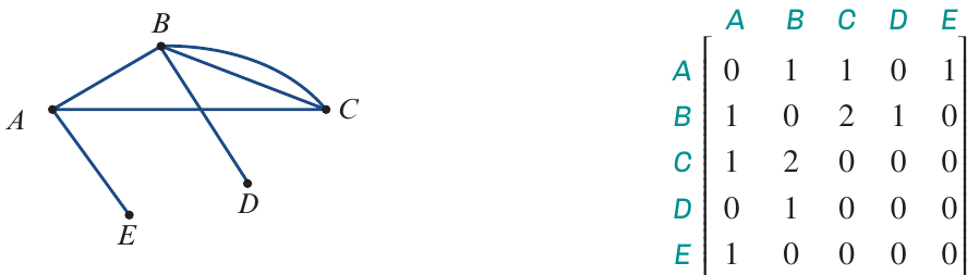
The diagram above shows both a graph and its corresponding adjacency matrix. Notice how the matrix captures all the same connection information as the visual graph, but in numerical form.

Structure of an adjacency matrix

The structure of an adjacency matrix follows specific rules that make it systematic and predictable.

Size and dimensions: If a graph has n vertices, its adjacency matrix will be an n × n square matrix. This means it has the same number of rows as columns. This square structure isn't arbitrary—it's necessary because we need to record potential connections from every vertex to every other vertex, including itself.

Row and column labels: Both the rows and columns are labelled with the vertex names (such as $A$ , $B$ , $C$ , $D$ , $E$ ). This creates a grid where you can find the connection between any two vertices by looking at where their row and column meet.

Understanding the entries: Each cell in the matrix contains a number that tells us how many edges connect those two vertices. The entry in the cell where row $X$ meets column $Y$ shows the number of edges between vertex X and vertex Y.

For example, if the adjacency matrix has these key features:

The matrix has five rows and five columns (one for each vertex)
Row and column labels match the vertices: $A$ , $B$ , $C$ , $D$ , $E$
Each intersection point contains a number showing the edge count

infoNote

Symmetry in Adjacency Matrices:

For undirected graphs (the most common type in introductory courses), the adjacency matrix is always symmetric. This means the entry at row $A$ , column $B$ equals the entry at row $B$ , column $A$ . This makes sense because an edge connecting $A$ to $B$ is the same as an edge connecting $B$ to $A$ .

Reading an adjacency matrix

Understanding what each number means in an adjacency matrix is essential for working with graphs. Let's explore the different values you'll encounter:

Zero entries (no connection): A 0 in the cell where row $A$ meets column $D$ means there is no edge connecting vertex $A$ to vertex $D$ . Similarly, a $0$ where row $A$ meets column $A$ means there is no loop at vertex $A$ (no edge from $A$ back to itself).

Single edge: A 1 in the cell where row $A$ meets column $B$ indicates there is exactly one edge connecting vertex $A$ to vertex $B$ .

Multiple edges: A 2 in the cell where row $C$ meets column $B$ shows there are two separate edges connecting vertex $C$ to vertex $B$ . When a graph has multiple edges between the same pair of vertices, we call it a multigraph.

Pattern for all connections: Every other pair of vertices in the graph is recorded in the adjacency matrix following the same pattern. To find out how many edges connect any two vertices, simply locate where their row and column intersect and read the number.

chatImportant

Common Mistake to Avoid:

Students sometimes confuse the position in the matrix with the number of edges. Remember: the position (row and column) tells you which vertices you're looking at, while the number in that cell tells you how many edges connect them. Always check both the row label and the column label before reading the entry.

Converting from adjacency matrix to graph

Sometimes you'll be given an adjacency matrix and need to draw the corresponding graph. This process involves systematically working through the matrix to recreate all the connections.

lightbulbExample

Worked Example: Drawing a graph from an adjacency matrix

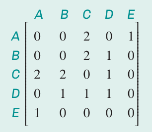
Question: Draw the graph represented by the following adjacency matrix.

Solution:

Step 1: Create and label the vertices

Begin by drawing a dot for each vertex and labelling them $A$ to $E$ . At this stage, don't add any edges yet—just establish the five vertices. This gives you a clear starting point before dealing with connections.

Step 2: Add edges based on matrix entries

Work through the matrix systematically. For instance:

The cell at row $A$ , column $C$ contains a $2$
This means we need two edges connecting vertex $A$ to vertex $C$
Add these two edges to your graph

Step 3: Identify and add loops

Check the diagonal of the matrix (where row and column labels match):

The cell at row $D$ , column $D$ contains a $1$
This shows there is a loop at vertex D
Draw this loop as an edge that starts and ends at vertex $D$

Step 4: Complete all remaining edges

Continue examining every intersection of row and column in the matrix. Add the appropriate number of edges to your graph for each non-zero entry. Make sure you don't duplicate edges you've already drawn.

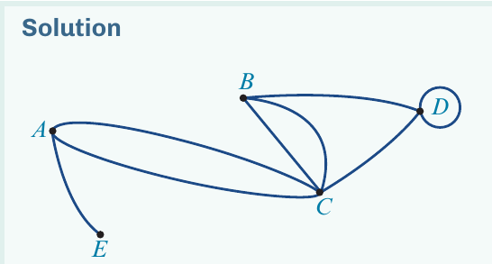
Note that this graph can be drawn in various ways. The solution shows it as a planar graph (with no edges crossing), but other arrangements are equally valid as long as all the connections match the adjacency matrix.

The key to success with matrix-to-graph conversion is being systematic. Don't try to draw everything at once—work through the matrix methodically, and you'll avoid missing connections or adding extras.

Converting from graph to adjacency matrix

The reverse process—creating an adjacency matrix from a given graph—is equally important. This involves systematically recording the connections you see in the visual graph. The advantage of this direction is that you can visually count the edges, making it often more straightforward than going from matrix to graph.

lightbulbExample

Worked Example: Creating an adjacency matrix

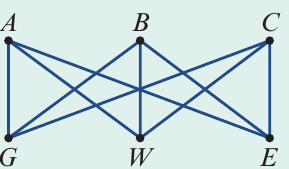
Question: Construct an adjacency matrix to represent the graph shown below. This graph shows how three houses ( $A$ , $B$ , $C$ ) connect to three utility outlets: gas ( $G$ ), water ( $W$ ), and electricity ( $E$ ).

Solution:

To create the adjacency matrix, follow these steps:

Step 1: Set up the matrix structure

Create a $6 \times 6$ matrix (since there are six vertices). Label both the rows and columns with all vertex names: $A$ , $B$ , $C$ , $G$ , $W$ , $E$ .

Step 2: Fill in the entries

For each pair of vertices, count the number of edges connecting them and enter this number in the appropriate cell. The completed adjacency matrix is:

	A	B	C	G	W	E
A	0	0	0	1	1	1
B	0	0	0	1	1	1
C	0	0	0	1	1	1
G	1	1	1	0	0	0
W	1	1	1	0	0	0
E	1	1	1	0	0	0

Understanding the pattern: Notice how this matrix shows that:

Each house connects to each utility outlet (shown by $1$ s)
No house connects to another house (shown by $0$ s in the top-left section)
No utility connects to another utility (shown by $0$ s in the bottom-right section)

This type of graph is called a bipartite graph because the vertices are divided into two distinct groups (houses and utilities), and edges only connect vertices from different groups, never within the same group.

This example demonstrates a practical application of graphs and matrices. The classic "utilities problem" asks whether you can connect all houses to all utilities without any lines crossing—a question that becomes easier to analyze using the adjacency matrix representation.

Key definitions and concepts

Understanding these formal definitions will help consolidate your knowledge of adjacency matrices and prepare you for exam questions.

chatImportant

Formal Definition: Adjacency Matrix

The adjacency matrix $A$ of a graph is an n × n matrix in which the entry in any row and column (for example, row $C$ and column $F$ ) represents the number of edges joining those two vertices (in this case, vertices $C$ and $F$ ).

Loop: A loop is a single edge that connects a vertex to itself. On a graph, a loop appears as an edge that starts and ends at the same vertex.

How loops appear in adjacency matrices: Loops are counted as one edge. In the adjacency matrix, a loop at vertex $X$ is shown as a $1$ in the cell where row $X$ meets column $X$ (the diagonal of the matrix).

infoNote

Diagonal Entries:

The diagonal of an adjacency matrix (from top-left to bottom-right) always represents potential loops. A non-zero entry on the diagonal means that vertex has a loop, while a zero means it doesn't. This is one of the first things to check when reading an adjacency matrix.

Bipartite graph: A bipartite graph is one where the set of vertices can be separated into two distinct groups, and each edge connects a vertex from one group to a vertex in the other group. No edges connect vertices within the same group.

chatImportant

Exam Tip:

When creating an adjacency matrix, always check that it's symmetric (the value at row $A$ , column $B$ equals the value at row $B$ , column $A$ ) unless you're working with a directed graph. For simple undirected graphs, this symmetry should always hold. If your matrix isn't symmetric, you've made an error somewhere—go back and check your edge counting.

Remember!

bookmarkSummary

Key Points to Remember:

An adjacency matrix is an n × n matrix where $n$ is the number of vertices in the graph
The entry at row $X$ , column $Y$ shows the number of edges connecting vertices $X$ and $Y$
A value of 0 means no connection exists between those vertices
Loops appear on the diagonal of the matrix (where row and column labels match)
To convert a matrix to a graph: create vertices first, then add edges according to the matrix entries
In a bipartite graph, vertices split into two groups with edges only between groups, never within them
Always check for symmetry in undirected graphs—it's a quick way to verify your work

Adjacency Matrices (VCE SSCE General Mathematics): Revision Notes