Matching and Allocation Problems (VCE SSCE General Mathematics): Revision Notes
Matching and Allocation Problems
Introduction to bipartite graphs
A bipartite graph is a special type of graph where the vertices are divided into two separate groups. The key characteristic is that each edge connects a vertex from one group to a vertex in the other group. In other words, edges never connect vertices within the same group.
Key Characteristic of Bipartite Graphs:
Each edge in a bipartite graph joins a vertex from one group to a vertex in the other group. Vertices within the same group are never connected to each other.
Understanding bipartite graphs through an example
Imagine a music school with four teachers: Anastasios, Panayioti, Olga, and Irene. These teachers can teach four different musical instruments: trumpet, piano, violin, and clarinet. We can represent this situation using a bipartite graph.
In the graph:
- One group contains the four teachers (shown as vertices on the left)
- The other group contains the four instruments (shown as vertices on the right)
- Edges connect each teacher to the instruments they are qualified to teach
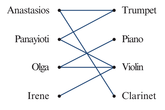
This visual representation helps us see which teachers can teach which instruments at a glance. The edges show the possible connections, making it easier to solve allocation problems.
Solving allocation problems with bipartite graphs
An allocation problem involves matching items from one group to items in another group. In the music school example, we need to assign each teacher to exactly one instrument class.
By examining the bipartite graph, we can work out the optimal allocation:
- Anastasios is the only teacher who can teach clarinet, so he must be assigned to clarinet
- Irene can only teach violin, so she must be assigned to violin
- With those two assignments made, Olga must teach piano
- Finally, Panayioti must teach trumpet
This logical process of elimination allows us to find a complete allocation where each teacher has one class and each instrument has one teacher.
Worked example: TV presenters
Worked Example: Allocating TV Presenters to Countries
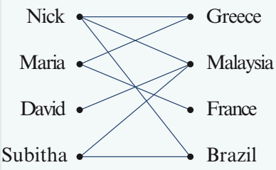
Problem: Nick, Maria, David, and Subitha are presenters on a TV travel show. Each presenter will be assigned to film a story about one country they have visited before. The countries they have visited are:
- Nick: Greece, Malaysia, and Brazil
- Maria: Greece and France
- Subitha: Malaysia and Brazil
- David: Malaysia
Step 1: Construct a bipartite graph
Create two groups of vertices:
- Left group: The four presenters (Nick, Maria, David, Subitha)
- Right group: The countries (Greece, Malaysia, France, Brazil)
Draw edges connecting each presenter to the countries they have visited.
Step 2: Identify forced allocations
Look for vertices with only one edge:
- David has only visited Malaysia, so he must be assigned to Malaysia
- France has only been visited by Maria, so Maria must be assigned to France
Step 3: Use elimination to complete the allocation
Since Maria is assigned to France, she cannot visit Greece. Nick is the only remaining presenter who has visited Greece, so Nick must be assigned to Greece.
With David assigned to Malaysia, Subitha has only Brazil remaining as an option, so Subitha must be assigned to Brazil.
Final allocation:
- Nick → Greece
- Maria → France
- David → Malaysia
- Subitha → Brazil
Complete bipartite graphs
A complete bipartite graph is a special case where every vertex in one group is connected to every vertex in the other group. This means there are edges between all possible pairs of vertices from different groups.
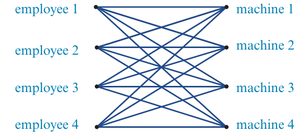
In the factory example shown above, there are four employees and four machines. Each employee can use every machine, so every employee vertex connects to every machine vertex. This creates a complete bipartite graph.
When every vertex connects to every other vertex in the opposite group, we cannot simply use the visual method from earlier to find the optimal allocation. Instead, we need additional information and a systematic algorithm.
The Hungarian algorithm
Introduction to cost matrices
In real-world allocation problems, some matches are better than others. For example, different employees might take different amounts of time to complete tasks on different machines. We can represent this information in a cost matrix.
A cost matrix is a table where:
- Rows represent items from the first group (e.g., employees)
- Columns represent items from the second group (e.g., machines)
- Each cell contains the "cost" of that particular allocation (e.g., time in minutes)
Here's an example cost matrix for a factory with four employees (Wendy, Xenefon, Yolanda, and Zelda) and four machines (A, B, C, and D):
| Employee | A | B | C | D |
|---|---|---|---|---|
| Wendy | 30 | 40 | 50 | 60 |
| Xenefon | 70 | 30 | 40 | 70 |
| Yolanda | 60 | 50 | 60 | 30 |
| Zelda | 20 | 80 | 50 | 70 |
The numbers represent how many minutes each employee takes to complete their task on each machine. For instance, Wendy takes minutes on machine A but minutes on machine D.
Purpose of the Hungarian algorithm
The Hungarian algorithm is a systematic method that finds the optimal allocation to minimise the total cost. It works by transforming the cost matrix through a series of steps until we can identify the best allocation.
The algorithm ensures that we assign each employee to exactly one machine (or each item from one group to exactly one item from the other group) while minimising the total time, cost, or whatever metric we're measuring.
Steps of the Hungarian algorithm
Step 1: Row reduction
Subtract the smallest value in each row from every value in that row.
This creates at least one zero in each row while preserving the relative differences within each row.
For our example:
- Wendy's row: subtract from each value
- Xenefon's row: subtract from each value
- Yolanda's row: subtract from each value
- Zelda's row: subtract from each value
| Employee | A | B | C | D |
|---|---|---|---|---|
| Wendy | 0 | 10 | 20 | 30 |
| Xenefon | 40 | 0 | 10 | 40 |
| Yolanda | 30 | 20 | 30 | 0 |
| Zelda | 0 | 60 | 30 | 50 |
Step 2: Check if we can allocate
Count the minimum number of straight lines (horizontal or vertical) needed to cover all the zeros in the table.
If this number equals the number of allocations to be made, jump to Step 6.
Otherwise, continue to Step 3.
In our example, we need three lines to cover all zeros, but we need to make four allocations. Therefore, we continue.
Step 3: Column reduction
If any column does not contain a zero, subtract the smallest value in that column from every value in that column.
Column C doesn't have a zero, so subtract from every value in column C:
| Employee | A | B | C | D |
|---|---|---|---|---|
| Wendy | 0 | 10 | 10 | 30 |
| Xenefon | 40 | 0 | 0 | 40 |
| Yolanda | 30 | 20 | 20 | 0 |
| Zelda | 0 | 60 | 20 | 50 |
Step 4: Check again
Count the minimum number of lines needed to cover all zeros.
If this equals the number of allocations, jump to Step 6.
Otherwise, continue to Step 5a.
We still need only three lines to cover all zeros, so we continue.
Step 5a: Adjust uncovered values
Find the smallest uncovered value (value not covered by any line).
Then:
- Add this value to any cell covered by two lines
- Subtract this value from all uncovered cells
- Leave cells covered by one line unchanged
In our example, the smallest uncovered value is .
Add to cells covered by two lines and subtract from uncovered cells:
| Employee | A | B | C | D |
|---|---|---|---|---|
| Wendy | 0 | 0 | 0 | 30 |
| Xenefon | 50 | 0 | 0 | 50 |
| Yolanda | 30 | 10 | 10 | 0 |
| Zelda | 0 | 50 | 10 | 50 |
Step 5b: Repeat from Step 4
Check again how many lines are needed to cover all zeros.
Now we need four lines, which equals our four required allocations, so we proceed to Step 6.
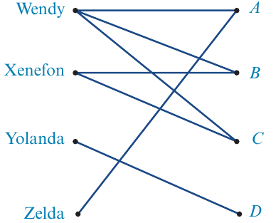
Step 6: Draw bipartite graph
Create a bipartite graph with an edge for every zero in the final table.
From our final table:
- Wendy connects to A, B, and C (has zeros in those columns)
- Xenefon connects to B and C
- Yolanda connects to D
- Zelda connects to A
Step 7: Make allocation and calculate minimum cost
Using the bipartite graph, determine the allocation by looking for forced assignments.
Critical: Always use the original cost matrix to calculate the final total cost, not the transformed matrix.
Worked Example: Final Allocation and Cost Calculation
Using the bipartite graph, determine the allocation by looking for forced assignments:
- Zelda can only connect to A (only one edge), so Zelda → machine A
- Yolanda can only connect to D, so Yolanda → machine D
- Wendy and Xenefon can both connect to B or C
For the remaining choices, select one valid allocation. Both options will give the same minimum cost.
Let's choose: Wendy → machine B and Xenefon → machine C
Now calculate the total cost using the original cost matrix:
- Zelda on machine A: minutes
- Yolanda on machine D: minutes
- Wendy on machine B: minutes
- Xenefon on machine C: minutes
Total minimum time: minutes
Exam tips
When performing the Hungarian algorithm:
- Always work carefully through each step in order
- Keep track of which operation you're performing (row reduction, column reduction, etc.)
- When covering zeros with lines, use the minimum number possible
- Double-check your arithmetic at each stage
- Remember to use the original cost matrix when calculating the final total cost
- Show all your working clearly in the exam
Key Points to Remember:
- Bipartite graphs have vertices in two separate groups, with edges only connecting vertices from different groups
- Allocation problems can be solved by identifying forced assignments (vertices with only one connection) and using elimination
- Complete bipartite graphs occur when every vertex in one group connects to every vertex in the other group
- The Hungarian algorithm finds the optimal allocation that minimises total cost through systematic row reduction, column reduction, and adjustment steps
- Always use the original cost matrix to calculate the final minimum cost, not the transformed matrix from the algorithm