Comparing the Distribution of a Numerical Variable Across Groups Revision Notes for VCE SSCE General Mathematics

Comparing the Distribution of a Numerical Variable Across Groups

Understanding the comparison

When we compare data distributions, we're looking at how the same measurement varies across different groups. This is meaningful when we measure the same numerical variable for different categories of people or things.

For example, we might want to compare:

Maximum daily temperatures in Melbourne during March with those in Sydney during March
Test scores of students who attended a revision class with those who did not

In each case, we're working with two types of variables:

A numerical variable (the measurement being taken, such as temperature or test score)
A categorical variable (the grouping, such as city or attendance at revision class)

infoNote

When we compare distributions across groups, we're actually investigating the relationship between a numerical variable and a categorical variable. This is a fundamental concept in statistics that helps us understand how measurements differ between groups.

Methods for comparing distributions

There are two main graphical methods for comparing distributions:

Back-to-back stem plots: Best for comparing two small data sets
Parallel boxplots: Can be used for two or more groups, and works well with larger data sets

Both methods help us compare distributions by examining their centre, spread, and any outliers.

Comparing distributions using back-to-back stem plots

What is a back-to-back stem plot?

A back-to-back stem plot is different from a regular stem plot because it has:

One central stem (the tens digits)
Two sets of leaves (the units digits), one on each side
Each set of leaves represents data from one of the two groups being compared

Reading a back-to-back stem plot

In a back-to-back stem plot:

The stem sits in the middle
One group's data appears on the left side
The other group's data appears on the right side
Each leaf represents one data value

lightbulbExample

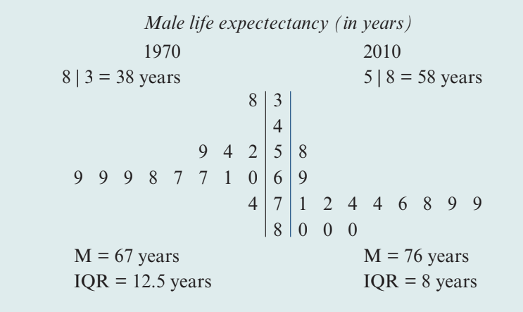
Worked Example: Comparing Male Life Expectancy

Consider male life expectancy data from several countries in 1970 and 2010:

Male life expectancy (in years)

Solution:

Step 1 - Compare centre:

The median life expectancy of males in 2010 ( $M = 76$ years) was higher than in 1970 ( $M = 67$ years).

Step 2 - Compare spread:

The spread of life expectancies of males in 2010 ( $\text{IQR} = 8$ years) was lower than the spread in 1970 ( $\text{IQR} = 12.5$ years).

Step 3 - Write a conclusion:

In conclusion, the median life expectancy for men in these countries has increased over the last 40 years, and the variability in male life expectancy has decreased over this time interval.

Writing a comparison

When comparing distributions using back-to-back stem plots, follow these three key steps:

Compare centre: Write a sentence using the medians
Compare spread: Write a sentence using the IQRs
Write a conclusion: Use your observations to add a general conclusion in context

chatImportant

Exam Tip

Always use comparative language such as "higher than," "lower than," "greater than," or "less than" when comparing statistics. Don't just state the values without comparison.

Comparing distributions using parallel boxplots

What are parallel boxplots?

Parallel boxplots are multiple boxplots drawn on the same axis, allowing easy visual comparison of:

Centre (median)
Spread (IQR)
Outliers

Advantages of parallel boxplots

Unlike back-to-back stem plots, parallel boxplots:

Can compare more than two groups
Work well with larger data sets
Provide immediate visual comparison of key features

Key features to compare

When using parallel boxplots to compare distributions, your report should address three essential features:

Centre: Compare the medians (the vertical lines inside the boxes)
Spread: Compare the IQRs (the widths of the boxes)
Outliers: Identify any outliers (shown as individual points beyond the whiskers)

lightbulbExample

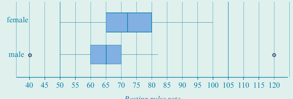
Worked Example: Comparing Pulse Rates

The following parallel boxplots show the distribution of resting pulse rates (in beats per minute) for female and male students:

Solution:

Step 1 - Compare centre:

The median pulse rate for females ( $M = 72$ beats/minute) is higher than that for males ( $M = 65$ beats/minute).

Step 2 - Compare spread:

The spread of pulse rates for females ( $\text{IQR} = 15$ ) is higher than for males ( $\text{IQR} = 10$ ).

Step 3 - Identify outliers:

There are no female pulse rate outliers. The males with pulse rates of 40 and 120 were outliers.

Step 4 - Write a conclusion:

In conclusion, the median pulse rate for females was higher than for males, and female pulse rates were generally more variable than male pulse rates.

Practice example: Exam time

The following parallel boxplots display the time (in minutes) spent in an exam by female and male students:

infoNote

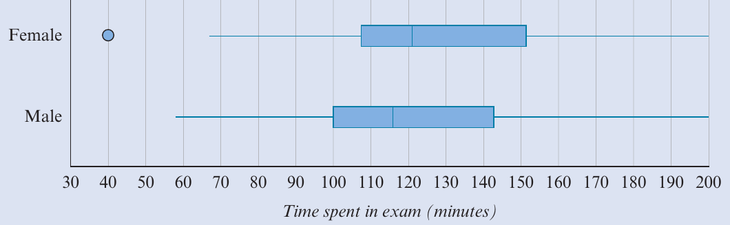
When comparing these distributions, remember to:

Compare the medians to discuss centre
Compare the IQRs to discuss spread
Identify any outliers
Write a clear, informative conclusion in context

Summary

bookmarkSummary

Key Points to Remember:

Comparing numerical distributions across groups investigates the relationship between a numerical variable and a categorical variable
Back-to-back stem plots are suitable when:
- There are only two groups
- The data sets are small
Parallel boxplots are suitable when:
- There are two or more groups
- The data sets are larger
Data distributions should always be compared in terms of:
- Centre: Quote the median for each group
- Spread: Quote the IQR for each group
- Outliers: Mention the values of any outliers
Your comparison should include clear comparative statements and a conclusion written in the context of the data

Remember!

chatImportant

Essential Guidelines for Comparing Distributions:

When comparing distributions, you're investigating the relationship between a numerical variable and a categorical variable
Use back-to-back stem plots for two small data sets
Use parallel boxplots for larger data sets or when comparing more than two groups
Always address three features: centre (median), spread (IQR), and outliers
Use comparative language ("higher than," "lower than") rather than just stating values
End with a clear conclusion that relates to the context of the data

Comparing the Distribution of a Numerical Variable Across Groups (VCE SSCE General Mathematics): Revision Notes