The Five-Number Summary and the Boxplot Revision Notes for VCE SSCE General Mathematics

The Five-Number Summary and the Boxplot

Introduction to the five-number summary

When analyzing data, knowing just the median and quartiles tells us about the centre and spread of a distribution. However, to get a complete picture of the distribution, we also need information about the extreme values (the tails). This is where the five-number summary becomes useful.

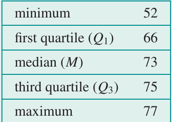
The five-number summary combines information about the centre, spread, and extremes of a data set into one concise summary. It consists of five key values arranged in order:

$\text{minimum}, \quad Q_1, \quad M, \quad Q_3, \quad \text{maximum}$

infoNote

The five-number summary provides a complete snapshot of your data's distribution in just five values. This concise format makes it perfect for quick comparisons between different data sets and forms the foundation for boxplot construction.

where:

Minimum is the smallest data value
$Q_1$ is the first quartile (lower quartile)
$M$ is the median (the middle value)
$Q_3$ is the third quartile (upper quartile)
Maximum is the largest data value

This summary provides the foundation for creating one of the most powerful tools in data analysis: the boxplot.

Understanding the boxplot

A boxplot (also called a box-and-whisker plot) is a graphical way to display the five-number summary. It provides a visual representation that makes it easy to see the distribution's shape, centre, spread, and any unusual values.

Components of a boxplot

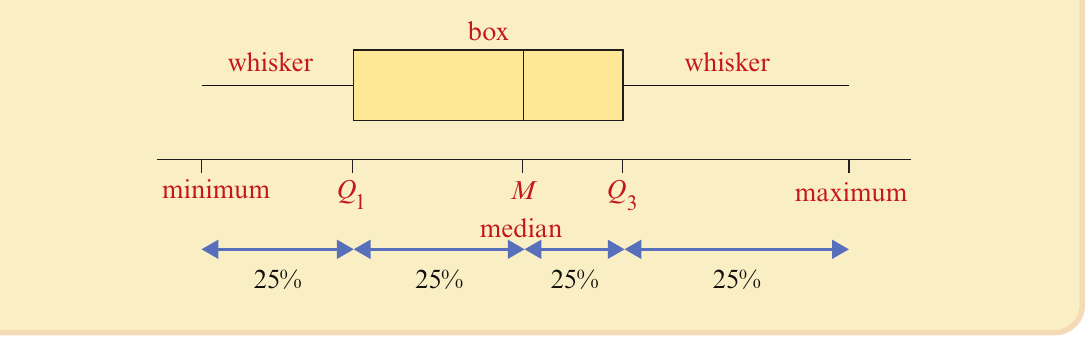
A boxplot consists of several key features:

The box: A rectangle that extends from $Q_1$ to $Q_3$ , containing the middle 50% of all data values
The median line: A vertical line inside the box marking the median position
The whiskers: Horizontal lines extending from each end of the box to the minimum and maximum values
Four equal sections: Each representing 25% of the data

Understanding what each part represents helps you interpret the distribution:

25% of values lie between the minimum and $Q_1$
25% of values lie between $Q_1$ and the median
25% of values lie between the median and $Q_3$
25% of values lie between $Q_3$ and the maximum

infoNote

Each quarter of a boxplot contains exactly the same number of data points, even though the physical lengths of the sections may differ. This is a key insight for understanding how data is distributed across the range.

Constructing a boxplot from a five-number summary

Let's work through an example to understand how to create a boxplot from a five-number summary.

Worked example: Life expectancy data

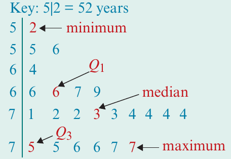
Consider the following five-number summary for life expectancies (in years) across 23 countries:

lightbulbExample

Worked Example: Constructing a Boxplot

Step 1: Draw a horizontal number line that covers the full range of values (from 50 to 80 years in this case). Make sure to label it clearly.

Step 2: Draw a rectangular box starting at $Q_1 = 66$ and ending at $Q_3 = 75$ .

Step 3: Mark the median value with a vertical line inside the box at $M = 73$ .

Step 4: Draw the whiskers by extending lines from the centre of each end of the box to the minimum value (52) and maximum value (77).

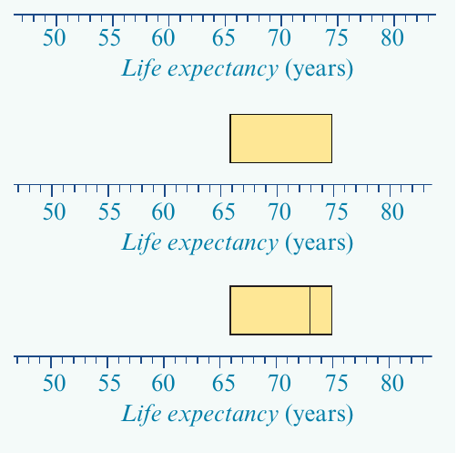
The completed boxplot gives you an immediate visual sense of how the life expectancies are distributed across these countries.

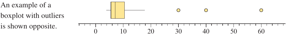
Boxplots with outliers

Sometimes a data set contains outliers – values that are unusually far from the rest of the data. A long whisker on a boxplot might indicate either extreme skewness or the presence of outliers. To distinguish between these situations, we need a precise definition of what counts as an outlier.

Defining outliers mathematically

chatImportant

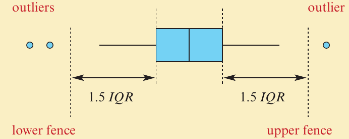
An outlier is any data value that lies more than 1.5 interquartile ranges beyond the quartiles. Specifically, a value is considered an outlier if it is:

Greater than $Q_3 + 1.5 \times IQR$ (upper outlier)
Less than $Q_1 - 1.5 \times IQR$ (lower outlier)

where $IQR = Q_3 - Q_1$ (the interquartile range).

Upper and lower fences

To identify outliers systematically, we use imaginary boundaries called fences:

Upper fence: $\text{Upper fence} = Q_3 + 1.5 \times IQR$

Lower fence: $\text{Lower fence} = Q_1 - 1.5 \times IQR$

Any data value beyond these fences is classified as a potential outlier.

infoNote

The choice of 1.5 as the multiplier for the IQR is not arbitrary – it's a statistical convention that provides a good balance between identifying truly unusual values and avoiding false positives. This standard is widely accepted in data analysis.

Drawing boxplots with outliers

When creating a boxplot that includes outliers:

Calculate the upper and lower fences
Identify which data values fall beyond these fences
Plot each outlier as an individual dot or circle
Draw the whiskers only to the smallest and largest values that are not outliers

This modified approach helps you see both the main body of the data and any unusual extreme values separately.

Using a CAS calculator to create boxplots

While you can construct boxplots by hand, using a CAS calculator makes the process much faster and ensures accuracy, especially when dealing with large data sets.

Example: Student marks data

Display the following set of 19 marks as a boxplot with outliers:

28, 21, 21, 3, 22, 31, 35, 26, 27, 33, 43, 31, 30, 34, 48, 36, 35, 23, 24

lightbulbExample

Worked Example: Using a TI-Nspire CAS

Start a new document and add a Lists & Spreadsheet page
Enter the data into a list called "marks"
Add a Data & Statistics page
Select "marks" as the variable for the x-axis
Change the plot type from dot plot to boxplot
Use the trace function to read key values

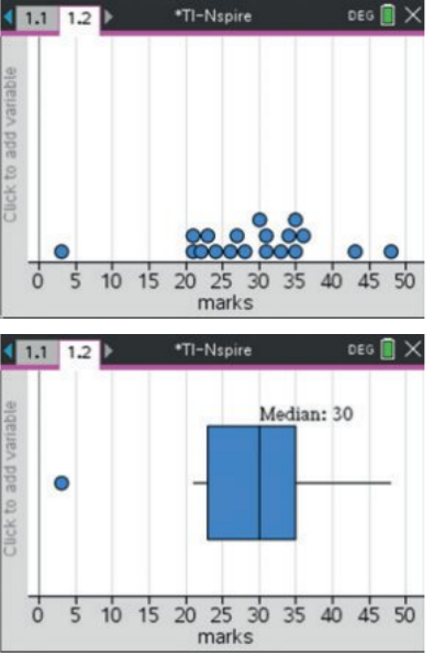
The calculator will automatically identify outliers and display them as separate dots. For this data set:

Minimum value: 3 (an outlier)
First quartile: $Q_1 = 23$
Median: $M = 30$
Third quartile: $Q_3 = 35$
Maximum value: 48

infoNote

Modern CAS calculators automatically apply the 1.5 IQR rule when identifying outliers, making the process faster and reducing calculation errors. However, you should still understand how to calculate fences manually for exam situations.

Reading and interpreting boxplots

Being able to extract information from a boxplot is just as important as creating one. Let's practice reading values and calculating statistics from boxplots.

Worked example: Reading values from a boxplot

lightbulbExample

Worked Example: Extracting Information from a Boxplot

For the boxplot shown, we can identify:

a) The median: $M = 36$ (the vertical line inside the box)

b) The quartiles: $Q_1 = 30$ and $Q_3 = 44$ (the ends of the box)

c) The interquartile range: $IQR = Q_3 - Q_1 = 44 - 30 = 14$

d) Minimum and maximum values: Minimum $= 4$ , Maximum $= 92$

e) Possible outliers: The dots show outliers at 4, 70, 84, and 92

f) Upper fence calculation:

\begin{aligned} \text{Upper fence} &= Q_3 + 1.5 \times IQR \\ &= 44 + 1.5 \times 14 \\ &= 44 + 21 = 65 \end{aligned}

Any value above 65 is classified as an outlier.

g) Lower fence calculation:

\begin{aligned} \text{Lower fence} &= Q_1 - 1.5 \times IQR \\ &= 30 - 1.5 \times 14 \\ &= 30 - 21 = 9 \end{aligned}

Any value below 9 is classified as an outlier.

Estimating percentages from boxplots

One of the powerful features of boxplots is that they allow you to estimate what percentage of data falls within certain ranges. This is because each section of the boxplot represents a specific percentage of the data.

Key percentage facts

25% of values are less than $Q_1$
50% of values are less than the median
75% of values are less than $Q_3$
25% of values are greater than $Q_3$

lightbulbExample

Worked Example: Percentage Calculations

For a boxplot with $Q_1 = 54$ , Median $= 55$ , $Q_3 = 59$ , and Maximum $= 86$ :

a) Percentage less than 54: Since 54 is $Q_1$ , 25% of values are less than 54.

b) Percentage less than 55: Since 55 is the median, 50% of values are less than 55.

c) Percentage less than 59: Since 59 is $Q_3$ , 75% of values are less than 59.

d) Percentage greater than 59: If 75% are less than 59, then 25% are greater than 59.

e) Percentage between 54 and 59: $75\% - 25\% = \mathbf{50\%}$

f) Percentage between 54 and 86: $100\% - 25\% = \mathbf{75\%}$

Relating boxplots to distribution shape

The shape of a boxplot reveals important information about how the data is distributed. By examining the position of the median within the box and the relative lengths of the whiskers, you can identify whether a distribution is symmetric or skewed.

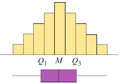
Symmetric distributions

A symmetric distribution has data values evenly spread around the median. Its boxplot characteristics include:

The median line is approximately in the centre of the box
The whiskers are roughly equal in length
The box appears balanced on either side of the median

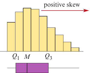
Positively skewed distributions

A positively skewed (or right-skewed) distribution has most data clustered toward the lower values, with a tail extending toward higher values. Its boxplot shows:

The median is positioned toward the left side of the box (closer to $Q_1$ )
The left whisker is short
The right whisker is long, reflecting the tail of higher values

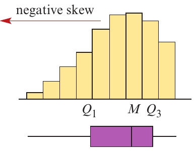
Negatively skewed distributions

A negatively skewed (or left-skewed) distribution has most data clustered toward the higher values, with a tail extending toward lower values. Its boxplot displays:

The median is positioned toward the right side of the box (closer to $Q_3$ )
The right whisker is short
The left whisker is long, reflecting the tail of lower values

chatImportant

A common mistake is to confuse the terms "positively skewed" and "negatively skewed" with the direction of the longer whisker. Remember: positively skewed means the tail extends toward the positive (right) direction, and negatively skewed means the tail extends toward the negative (left) direction.

Distributions with outliers

When a distribution contains outliers, the boxplot shows large gaps between the main body of data and extreme values. The box and whiskers represent the main data, while dots separated from them indicate outliers.

Using boxplots to describe distributions

Boxplots are extremely effective tools for describing the key features of a distribution. When analyzing a boxplot, you should comment on four main aspects: shape, centre, spread, and outliers.

Worked example: Positively skewed distribution

lightbulbExample

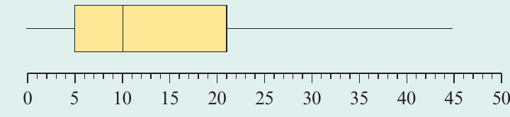
Worked Example: Describing a Positively Skewed Distribution

Description: The distribution is positively skewed with no outliers. The distribution is centred at 10 (the median value). The spread of the distribution, as measured by the IQR, is 16, and as measured by the range, is 45.

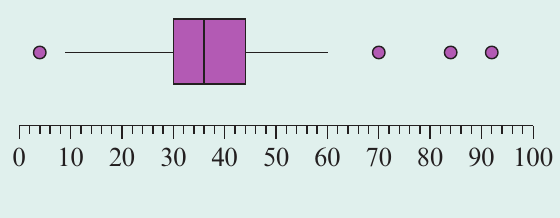
Worked example: Symmetric distribution with outliers

lightbulbExample

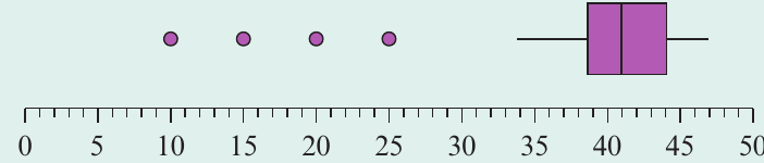
Worked Example: Describing a Symmetric Distribution with Outliers

Description: The distribution is symmetric but with outliers. The distribution is centred at 41 (the median value). The spread of the distribution, as measured by the IQR, is 5.5, and as measured by the range, is 37. There are four outliers: 10, 15, 20, and 25.

Worked example: Real-world application

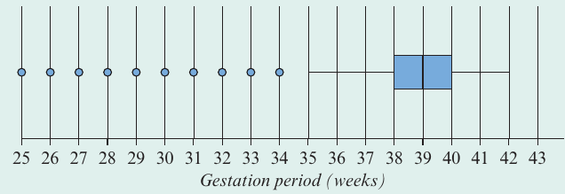
The boxplot shows the gestation period (completed weeks) for a sample of 1000 babies born in Australia.

lightbulbExample

Worked Example: Describing Real-World Data

Description: The distribution of gestational period is negatively skewed with several outliers. The distribution is centred at 39 weeks (the median value). The range of the distribution is 17 weeks, but the interquartile range is only 2 weeks. Any gestational period of 35 weeks or less is considered unusual, with outliers at 25, 26, 27, 28, 29, 30, 31, 32, 33, and 34 weeks.

infoNote

This example demonstrates why boxplots are so valuable in practical applications – they make it easy to identify both typical values and unusual cases that might need special attention. In medical contexts like this, outliers may represent cases requiring additional care or monitoring.

Exam tips

chatImportant

Critical Exam Tips

Always label your axes clearly when drawing boxplots, including units of measurement
Show your working when calculating fences for outliers: write out the formulas with substituted values
Check your quartile positions carefully – a common error is mixing up $Q_1$ and $Q_3$
Use the correct terminology in descriptions: use "positively skewed" not "skewed to the right"
Remember the 1.5 IQR rule for identifying outliers – this is the standard definition
When describing distributions, always address all four features: shape, centre, spread, and outliers

Remember!

bookmarkSummary

Key Points to Remember:

The five-number summary consists of: minimum, $Q_1$ , median, $Q_3$ , and maximum
A boxplot visually displays the five-number summary, with the box representing the middle 50% of data
Outliers are values more than $1.5 \times IQR$ beyond the quartiles
Upper fence = $Q_3 + 1.5 \times IQR$ and Lower fence = $Q_1 - 1.5 \times IQR$
Each quarter of a boxplot contains 25% of the data values
The shape of a distribution can be determined from boxplot features: symmetric distributions have centered medians and equal whiskers, while skewed distributions show off-center medians and unequal whiskers

The Five-Number Summary and the Boxplot (VCE SSCE General Mathematics): Revision Notes