The Normal Distribution and the 68–95–99.7% Rule Revision Notes for VCE SSCE General Mathematics

The Normal Distribution and the 68–95–99.7% Rule

Understanding the normal distribution

While we know that the interquartile range represents the spread of the middle $50\%$ of a data set, we need a similar way to interpret the standard deviation. We can do this for symmetric distributions that have an approximate bell shape. Although this might seem restrictive, many data distributions in statistics can be well approximated by this type of distribution, known as the normal distribution.

The normal distribution is remarkably common in real-world data. Many data sets arising in practice are roughly symmetrical and have approximate bell shapes.

infoNote

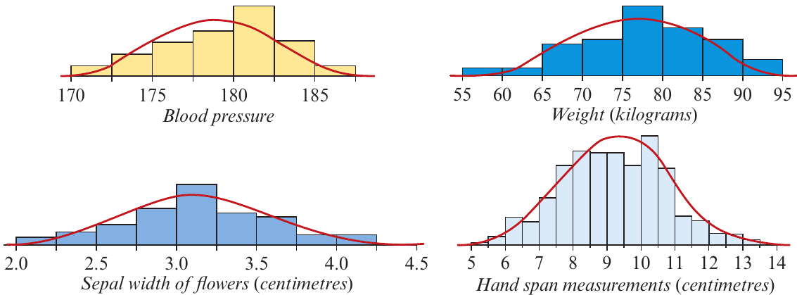
Key definition: Data distributions that are bell-shaped can be modelled by a normal distribution.

The 68–95–99.7% rule

For normal distributions, we can always determine the percentage of observations that lie within a certain number of standard deviations of the mean. This is particularly useful for understanding how data is spread around the mean.

The rule explained

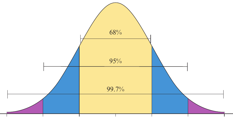
For a normal distribution, approximately:

$68\%$ of the observations lie within one standard deviation of the mean, in the interval $(\bar{x} - s, \bar{x} + s)$
$95\%$ of the observations lie within two standard deviations of the mean, in the interval $(\bar{x} - 2s, \bar{x} + 2s)$
$99.7\%$ of the observations lie within three standard deviations of the mean, in the interval $(\bar{x} - 3s, \bar{x} + 3s)$

chatImportant

This rule is one of the most powerful tools in statistics for understanding how data is distributed. Memorizing these three percentages—68, 95, and 99.7—will help you quickly interpret and analyze normally distributed data.

Visual representation

The following diagram shows these three key percentages:

Understanding the tails

Since the normal distribution is symmetrical and $100\%$ of observations lie within the curve, we can use the 68–95–99.7% rule to allocate percentages to the tails of the distribution.

Within one standard deviation:

Since around $68\%$ of data values lie within one standard deviation of the mean, approximately 16% of values lie in each of the tails.

Within two standard deviations:

Since around $95\%$ of data values lie within two standard deviations of the mean, approximately 2.5% of values lie in each of the tails.

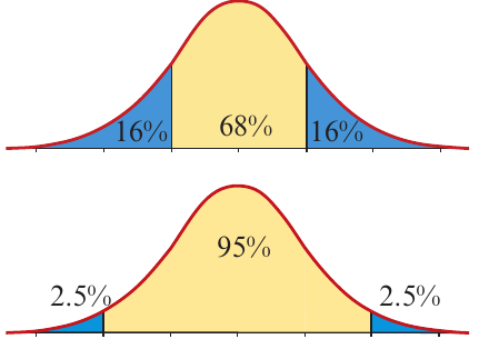
Within three standard deviations:

Since around $99.7\%$ of data values lie within three standard deviations of the mean, approximately 0.15% of values lie in each of the tails.

Complete percentage breakdown

When we combine all this information, we can allocate percentages to each section of the normal curve:

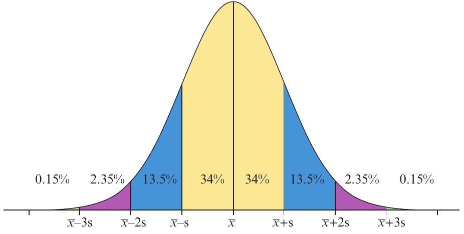
This detailed breakdown shows:

$0.15\%$ beyond three standard deviations (each tail)
$2.35\%$ between two and three standard deviations (each side)
$13.5\%$ between one and two standard deviations (each side)
$34\%$ within one standard deviation (each side of the mean)

infoNote

Notice how the percentages are perfectly symmetrical on both sides of the mean. This symmetry is a fundamental property of the normal distribution and makes it easier to work with.

Applying the 68–95–99.7% rule

Let's explore how to use this rule to solve practical problems.

lightbulbExample

Worked Example: Pizza Delivery Times

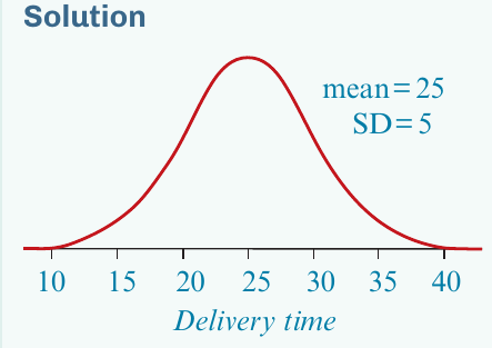
Problem: The distribution of delivery times for pizzas made by House of Pizza is approximately normal, with a mean of $25$ minutes and a standard deviation of $5$ minutes.

Part a: What percentage of pizzas have delivery times between $15$ and $35$ minutes?

Solution:

First, sketch and label a normal distribution curve with mean $= 25$ and standard deviation $= 5$ .

Next, shade the region representing delivery times between $15$ and $35$ minutes.

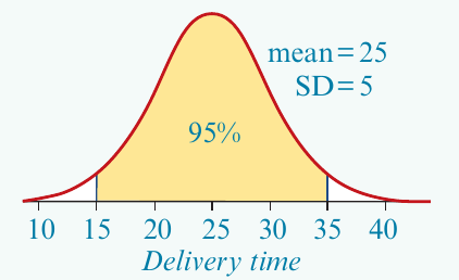
Note that:

$15 = 25 - 2 \times 5$ (two standard deviations below the mean)
$35 = 25 + 2 \times 5$ (two standard deviations above the mean)

Therefore, delivery times between $15$ and $35$ minutes lie within two standard deviations of the mean.

Using the 68–95–99.7% rule, $95\%$ of values are within two standard deviations of the mean.

Answer: 95% of pizzas will have delivery times between 15 and 35 minutes.

Part b: What percentage of pizzas have delivery times greater than $30$ minutes?

Solution:

Draw and label the distribution, shading the region for delivery times greater than $30$ minutes.

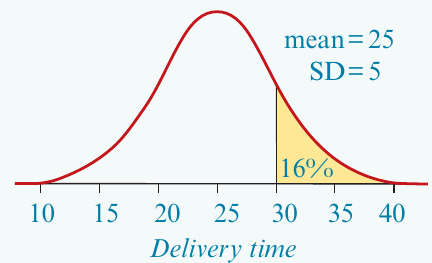
Note that:

$30 = 25 + 1 \times 5$ (one standard deviation above the mean)

Delivery times greater than $30$ minutes are more than one standard deviation above the mean. From our tail percentages, $16\%$ of values are more than one standard deviation above the mean.

Answer: 16% of pizzas will have delivery times greater than 30 minutes.

Part c: In one month, House of Pizza delivers $2000$ pizzas. Approximately how many are delivered in less than $10$ minutes?

Solution:

Total number of pizzas $= 2000$

Note that:

$10 = 25 - 3 \times 5$ (three standard deviations below the mean)

Delivery times less than $10$ minutes are more than three standard deviations below the mean. From the rule, $0.15\%$ of values are more than three standard deviations below the mean.

Number of pizzas delivered in less than $10$ minutes:

$= 0.15\% \text{ of } 2000$

$= \frac{0.15}{100} \times 2000 = 3$

Answer: Approximately 3 pizzas are delivered in less than 10 minutes.

Standard scores (z-scores)

The 68–95–99.7% rule makes the standard deviation a natural measuring tool for normally distributed data. By relating standard deviations to percentages, we gain additional insight into where a value sits within a distribution.

Why use standard scores?

Consider a person who scores $112$ on an IQ test with mean $100$ and standard deviation $15$ . This score is less than one standard deviation from the mean, placing them within the middle $68\%$ of scores (typical performance).

In contrast, someone scoring $133$ stands out significantly. Their score is more than two standard deviations from the mean, placing them in the top $2.5\%$ .

infoNote

Standard scores allow us to compare performances across different tests or distributions. A raw score alone doesn't tell us how exceptional a performance is—we need context from the mean and standard deviation.

What is a z-score?

We transform data into standardised scores (z-scores) to show how many standard deviations a value lies from the mean. This process is called standardising.

Calculating z-scores

To obtain a standard score from an actual score:

$z = \frac{x - \bar{x}}{s}$

where:

$z$ is the standardised score
$x$ is the actual score
$\bar{x}$ is the mean
$s$ is the standard deviation

Interpreting z-scores

A positive z-score indicates the actual score lies above the mean
A z-score of zero indicates the actual score equals the mean
A negative z-score indicates the actual score lies below the mean

chatImportant

The magnitude of the z-score tells us how unusual a value is. A z-score beyond $\pm 2$ indicates a value in the most extreme $5\%$ of the distribution, while a z-score beyond $\pm 3$ indicates a value in the most extreme $0.3\%$ .

lightbulbExample

Worked Example: Calculating z-scores

Problem: The heights of a group of young women have mean $\bar{x} = 160$ cm and standard deviation $s = 8$ cm. Determine the z-scores for women who are:

a) $172$ cm tall

Solution:

Given: $x = 172$ , $\bar{x} = 160$ , $s = 8$

$z = \frac{x - \bar{x}}{s} = \frac{172 - 160}{8} = \frac{12}{8} = 1.5$

b) $150$ cm tall

Solution:

Given: $x = 150$ , $\bar{x} = 160$ , $s = 8$

$z = \frac{x - \bar{x}}{s} = \frac{150 - 160}{8} = \frac{-10}{8} = -1.25$

c) $160$ cm tall

Solution:

Given: $x = 160$ , $\bar{x} = 160$ , $s = 8$

$z = \frac{x - \bar{x}}{s} = \frac{160 - 160}{8} = \frac{0}{8} = 0$

Using z-scores to compare performance

Standard scores are particularly useful for comparing groups with different means and/or standard deviations.

Comparing across different distributions

Consider a student with these marks:

Subject	Mark	Mean	Standard Deviation
Psychology	75	65	10
Statistics	70	60	5

At face value, the Psychology mark is higher. However, when we consider the different distributions, standardisation reveals the true picture.

Psychology z-score:

$z = \frac{75 - 65}{10} = \frac{10}{10} = 1$

Statistics z-score:

$z = \frac{70 - 60}{5} = \frac{10}{5} = 2$

Analysis

Although the student obtained a higher raw score for Psychology, she performed better relative to her classmates in Statistics:

Her Statistics mark (z-score $= 2$ ) was two standard deviations above the mean, placing her in the top 2.5% of students
Her Psychology mark (z-score $= 1$ ) was only one standard deviation above the mean, placing her in the top 16% of students

This demonstrates good performance in both subjects, but exceptional performance in Statistics.

infoNote

This example shows why comparing raw scores can be misleading. The z-score provides a fair comparison by accounting for both the mean and the variability in each distribution.

lightbulbExample

Worked Example: Equal Raw Scores

Problem: Another student obtained a mark of $55$ for both Psychology and Statistics. Does this mean she performed equally well in both subjects?

Solution:

Psychology:

Given: $x = 55$ , $\bar{x} = 65$ , $s = 10$

$z = \frac{x - \bar{x}}{s} = \frac{55 - 65}{10} = \frac{-10}{10} = -1$

Statistics:

Given: $x = 55$ , $\bar{x} = 60$ , $s = 5$

$z = \frac{x - \bar{x}}{s} = \frac{55 - 60}{5} = \frac{-5}{5} = -1$

Conclusion: Yes, her standardised score of z = -1 was the same for both subjects. In both subjects, she finished in the bottom $16\%$ of students.

Using z-scores with the normal curve

Once we understand z-scores, we can replace the horizontal scale on our normal curve diagram with z-score values:

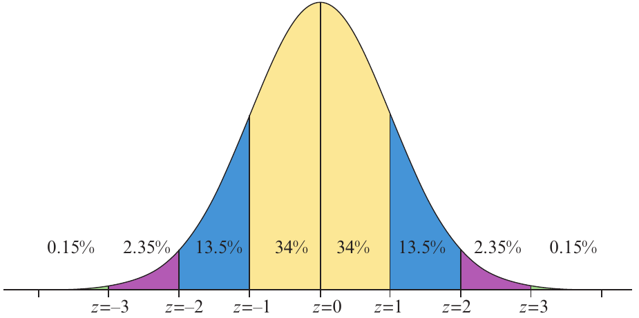
This standardised version shows the same percentage information, but uses z-scores instead of actual values.

infoNote

The standardised normal curve is universal—it applies to any normally distributed variable once we convert to z-scores. This makes it a powerful tool for analysis.

lightbulbExample

Worked Example: Determining Percentages with z-scores

Problem: The weight of a certain species of bird is normally distributed with mean $42$ grams and standard deviation $3$ grams.

Part a: If a randomly selected bird has standardised weight $z = -1$ , what percentage of birds weigh more than this bird?

Solution:

Locate $z = -1$ on the standardised normal curve. The percentage below $z = -1$ is $16\%$ .

Therefore, the percentage above $z = -1$ is:

$100\% - 16\% = 84\%$

Answer: 84% of birds weigh more than this bird.

Part b: What percentage of birds weigh between $39$ and $48$ grams?

Solution:

Given: $\bar{x} = 42$ , $s = 3$

For $x = 39$ :

$z = \frac{x - \bar{x}}{s} = \frac{39 - 42}{3} = \frac{-3}{3} = -1$

For $x = 48$ :

$z = \frac{x - \bar{x}}{s} = \frac{48 - 42}{3} = \frac{6}{3} = 2$

From the standardised curve, the percentage between $z = -1$ and $z = 2$ is:

$13.5\% + 34\% + 34\% = 81.5\%$

Answer: 81.5% of birds weigh between 39 and 48 grams.

Converting z-scores to actual scores

Sometimes we need to convert a standardised score back into an actual score.

The conversion formula

By rearranging the z-score formula, we get:

$x = \bar{x} + z \times s$

where:

$x$ is the actual score
$\bar{x}$ is the mean
$z$ is the standardised score
$s$ is the standard deviation

infoNote

This formula is the inverse operation of finding a z-score. Instead of standardising an actual score, we're converting a standardised score back to the original scale.

lightbulbExample

Worked Example: Converting z-scores

Problem: A class test (out of $50$ ) has mean mark $\bar{x} = 34$ and standard deviation $s = 4$ . Joe's standardised test mark was $z = -1.5$ . What was Joe's actual mark?

Solution:

Given: $\bar{x} = 34$ , $s = 4$ , $z = -1.5$

Using the formula:

$x = \bar{x} + z \times s$

$x = 34 + (-1.5) \times 4$

$x = 34 - 6 = 28$

Answer: Joe's actual mark was 28.

Finding unknown values

When we know percentages associated with a normal distribution, we can work backwards to find the mean or standard deviation (or both).

lightbulbExample

Worked Example: Finding Standard Deviation

Problem: The heights of red flowering gum trees have mean $10.2$ metres, and $2.5\%$ of these trees grow to more than $11.4$ metres tall. Assuming heights are approximately normally distributed, what is the standard deviation?

Solution:

Explanation	Solution
Since $2.5\%$ of trees are taller than $11.4$ metres, this height corresponds to a z-score of $2$	$\bar{x} = 10.2$ , $z = 2$
Write the rule for actual scores and substitute values	$x = \bar{x} + z \times s$ $11.4 = 10.2 + 2 \times s$
Solve for $s$	$2 \times s = 1.2$ $s = 0.6$ metres

Answer: The standard deviation is 0.6 metres.

chatImportant

When working backwards from percentages to find unknown values, the key step is identifying the correct z-score that corresponds to the given percentage. Use the 68–95–99.7% rule and the tail percentages to determine this.

lightbulbExample

Worked Example: Finding Both Mean and Standard Deviation

Problem: Examination marks are known to be approximately normally distributed. If $16\%$ of students score more than $80$ marks, and $2.5\%$ score less than $20$ marks, estimate the mean and standard deviation.

Solution:

Since $2.5\%$ of students score less than $20$ , this corresponds to $z = -2$ :

$\bar{x} - 2 \times s = 20 \quad \text{...(1)}$

Since $16\%$ of students score more than $80$ , this corresponds to $z = 1$ :

$\bar{x} + 1 \times s = 80 \quad \text{...(2)}$

Subtract equation $(1)$ from equation $(2)$ :

$-3 \times s = -60$

$s = 20$

Substitute $s = 20$ into equation $(1)$ :

$\bar{x} - 2 \times 20 = 20$

$\bar{x} = 60$

Answer: The mean is 60 and the standard deviation is 20.

bookmarkSummary

Key Points to Remember:

The normal distribution is a bell-shaped, symmetrical distribution that models many real-world data sets
The 68–95–99.7% rule tells us that approximately $68\%$ , $95\%$ , and $99.7\%$ of data lie within one, two, and three standard deviations of the mean respectively
Standardised scores (z-scores) show how many standard deviations a value lies from the mean, calculated using $z = \frac{x - \bar{x}}{s}$
Z-scores allow us to compare values across different distributions
We can convert z-scores back to actual scores using $x = \bar{x} + z \times s$
The 68–95–99.7% rule only applies to data that is approximately normally distributed

The Normal Distribution and the 68–95–99.7% Rule (VCE SSCE General Mathematics): Revision Notes