Sketching Graphs Revision Notes for VCE SSCE Mathematical Methods

Sketching Graphs

Introduction

The calculus techniques we use for sketching polynomial functions can also be applied to sketch more complex functions, including rational functions. By analyzing key features such as asymptotes, intercepts, and stationary points, we can create accurate graphs of non-polynomial functions.

infoNote

The same systematic approach we learned for polynomials—finding derivatives, locating stationary points, and analyzing behavior—works just as well for rational functions. We just need to add a few extra steps to handle asymptotes.

Worked example

lightbulbExample

Worked Example: Sketching a Rational Function

Let's sketch the graph of the function:

f: \mathbb{R} \setminus \{-1\} \to \mathbb{R}, \quad f(x) = \frac{x^2 + 3}{x + 1}

Step 1: Rewrite the function

When we perform polynomial division on the numerator and denominator, we can rewrite the function in a more useful form:

f(x) = x - 1 + \frac{4}{x + 1}

This form makes it easier to see the function's behavior and identify asymptotes.

Step 2: Determine behaviour for very large values of x

We need to examine what happens to the function as $x$ becomes very large in both the positive and negative directions.

As $x \to \infty$ , the term $\frac{4}{x+1}$ approaches zero, so $f(x) \to x - 1$ from above.

As $x \to -\infty$ , the term $\frac{4}{x+1}$ also approaches zero, so $f(x) \to x - 1$ from below.

This tells us there is an oblique asymptote with equation $y = x - 1$ . The graph will approach this slanted line but never quite reach it at extreme values.

chatImportant

An oblique asymptote (also called a slant asymptote) occurs when the graph approaches a non-horizontal, non-vertical line as $x$ approaches infinity. This happens when the degree of the numerator is exactly one more than the degree of the denominator.

lightbulbExample

Step 3: Find the vertical asymptote

A vertical asymptote occurs where the denominator of the original function equals zero. Setting $x + 1 = 0$ gives us $x = -1$ .

We can verify the behavior near this asymptote by checking the limits:

\lim_{x \to -1^+} f(x) = \infty \quad \text{and} \quad \lim_{x \to -1^-} f(x) = -\infty

Therefore, there is a vertical asymptote with equation $x = -1$ .

Step 4: Find axis intercepts

For the y-intercept, substitute $x = 0$ :

f(0) = \frac{0^2 + 3}{0 + 1} = 3

So the y-intercept is at $(0, 3)$ .

For x-intercepts, we would set $f(x) = 0$ , which requires $x^2 + 3 = 0$ . However, since $x^2 + 3 \neq 0$ for all real values of $x$ , there is no x-intercept.

Step 5: Find stationary points

To locate stationary points, we need to find where the first derivative equals zero.

Starting with $f(x) = x - 1 + \frac{4}{x + 1}$ , we differentiate:

f'(x) = 1 - \frac{4}{(x + 1)^2}

Setting $f'(x) = 0$ :

1 - \frac{4}{(x + 1)^2} = 0

(x + 1)^2 = 4

x + 1 = \pm 2

Therefore $x = 1$ or $x = -3$ .

Step 6: Classify the stationary points using sign charts

Since the function has a vertical asymptote at $x = -1$ that divides the domain into two separate regions, we need to create two sign charts to analyze the gradient on each side.

chatImportant

Why two sign charts?

The vertical asymptote at $x = -1$ splits the domain into two completely separate regions: $x > -1$ and $x < -1$ . The function cannot cross from one region to the other, so we must analyze the gradient behavior in each region independently.

lightbulbExample

For $x > -1$ :

Table

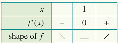
The derivative changes from negative to positive at $x = 1$ , indicating a local minimum at $(1, 2)$ .

To find the y-coordinate:

f(1) = \frac{1^2 + 3}{1 + 1} = \frac{4}{2} = 2

For $x < -1$ :

Table

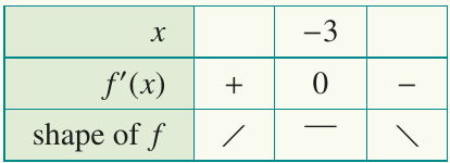
The derivative changes from positive to negative at $x = -3$ , indicating a local maximum at $(-3, -6)$ .

To find the y-coordinate:

f(-3) = \frac{(-3)^2 + 3}{-3 + 1} = \frac{12}{-2} = -6

Step 7: Sketch the graph

Now we can combine all the information to create our sketch:

Oblique asymptote: $y = x - 1$
Vertical asymptote: $x = -1$
Y-intercept: $(0, 3)$
Local minimum: $(1, 2)$
Local maximum: $(-3, -6)$

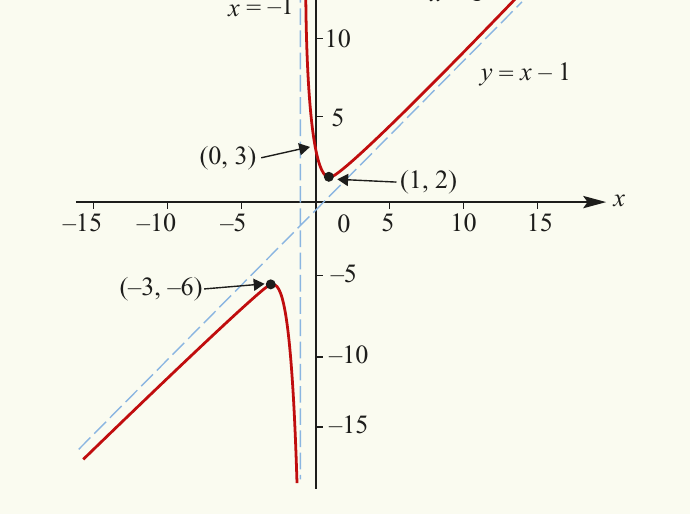
The graph shows two distinct branches separated by the vertical asymptote at $x = -1$ . Each branch approaches the oblique asymptote $y = x - 1$ as we move away from the origin, and each branch contains one stationary point.

Remember!

bookmarkSummary

Key Points for Sketching Rational Functions:

Rewrite rational functions using polynomial division to identify oblique asymptotes more easily
Vertical asymptotes occur where the denominator equals zero
Oblique asymptotes appear when the degree of the numerator is exactly one more than the degree of the denominator
Use sign charts to classify stationary points, especially when the function has vertical asymptotes that divide the domain into separate regions
Always label key features on your sketch: asymptotes, intercepts, and stationary points with their coordinates

Sketching Graphs (VCE SSCE Mathematical Methods): Revision Notes