Reciprocal and Modulus Graphs (AQA A-Level Further Maths): Revision Notes
Reciprocal and Modulus Graphs
Understanding reciprocal graphs
A reciprocal function is formed when you take the reciprocal of a function, written as . The graph of this reciprocal function has several important relationships with the original function .
Definition: The reciprocal of a function is , which is undefined wherever .
The values of where crosses the x-axis are called the roots or zeros of the function. These special points play a crucial role in reciprocal graphs.
The transformation from to creates a dramatically different graph with unique features. Understanding the relationship between these two graphs is essential for sketching reciprocal functions accurately.
Key properties of reciprocal graphs
When transforming into , several important changes occur to the graph:
Vertical asymptotes: The reciprocal function is undefined when . This means any roots or zeros of become vertical asymptotes in the graph of . The graph approaches these vertical lines but never touches or crosses them.
Critical Rule: Zeros Become Asymptotes
Wherever , the reciprocal function has a vertical asymptote. This is the most fundamental property of reciprocal graphs - roots transform into undefined points where the graph shoots off to infinity.
Behavior near asymptotes: Understanding what happens as the original function approaches zero is essential:
- When approaches 0 from above (from positive values), the reciprocal approaches positive infinity ()
- When approaches 0 from below (from negative values), the reciprocal approaches negative infinity ()
Sign relationship: The reciprocal function maintains the same sign as the original function. If is positive, then is also positive. If is negative, then is also negative.
Inverse gradient behavior: When the original function is increasing, the reciprocal decreases, and vice versa. This creates an inverse relationship in the slopes of the two graphs.
Understanding Inverse Behavior
Think of the gradient relationship like a seesaw: when goes up, goes down. This happens because as values get larger, their reciprocals get smaller, and vice versa.
Intersection points: When , the reciprocal also equals . At these points, the graphs of and intersect.
Turning points: Maximum points become minimum points and vice versa, with one important exception. If a turning point lies exactly on the x-axis (where ), it becomes a vertical asymptote instead of a turning point.
Range considerations: The size of determines the range of :
- If , then
- If , then
- If , then
- If , then
Range Relationships
When is large (greater than 1 or less than -1), its reciprocal is small (between -1 and 1). When is small (between -1 and 1), its reciprocal is large (outside the -1 to 1 range). This inverse size relationship helps you sketch the shape of reciprocal graphs.
Behavior at infinity: When approaches zero, approaches infinity. Conversely, when approaches infinity (becomes very large), approaches zero.
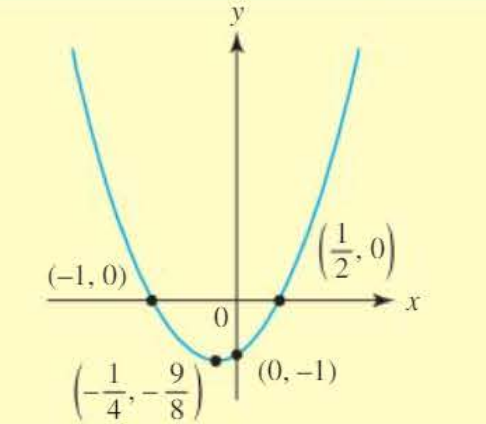
Worked example 1: Sketching a reciprocal graph from an equation
Worked Example: Quadratic Reciprocal Graph
Given:
a) Sketch the graph of
First, we identify the key features of this quadratic function:
- The y-intercept is at (substitute )
- To find x-intercepts, set :
- Factoring:
- x-intercepts are at and
To find the vertex, complete the square:
The minimum point is at .
b) On the same axes, sketch
Now we use the properties of reciprocal graphs to transform our sketch:
Step 1: Identify vertical asymptotes Since has roots at and , the reciprocal function will have vertical asymptotes at these values. The function is undefined at these points.
Step 2: Find intersection points We solve :
The graphs intersect at approximately and .
We also solve :
The graphs intersect at and .
Step 3: Analyze turning points and gradient
The minimum point of at becomes a maximum point of at the same x-coordinate.
Since is increasing for and decreasing for , the reciprocal decreases for and increases for .
Step 4: Determine signs
Both and are negative in the region , and positive elsewhere (excluding the asymptotes).
Worked example 2: Sketching from a given graph
Sometimes you need to sketch the reciprocal graph when you don't have the function equation, but you're given the graph of with labeled points.
Worked Example: Reciprocal from a Given Graph
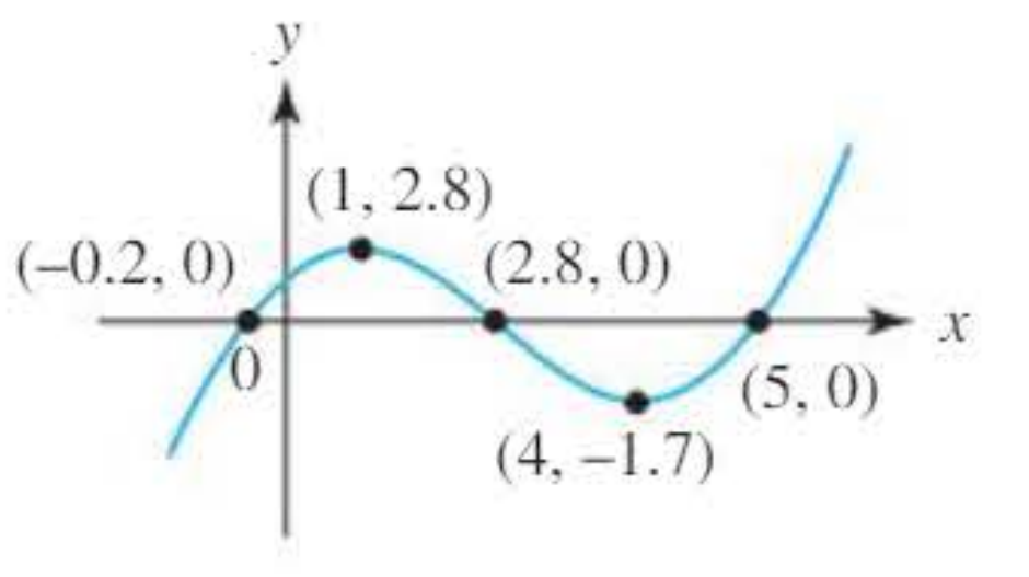
Given: A graph showing with key points at , , , a local maximum at , and a local minimum at .
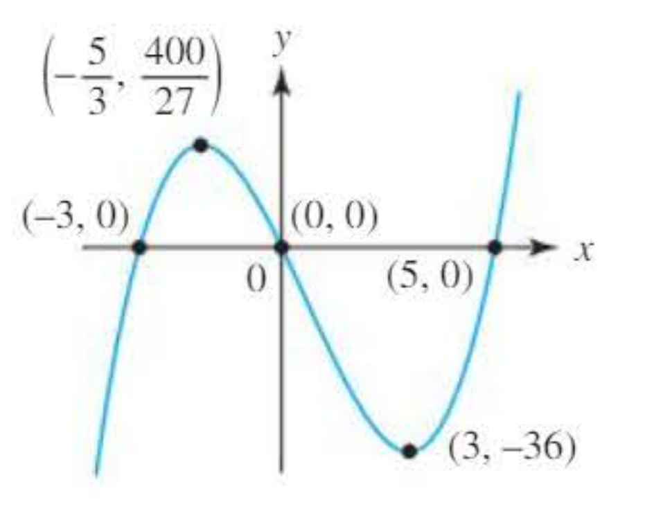
Solution:
Step 1: Identify vertical asymptotes The function has three roots at , , and . Therefore, will have three vertical asymptotes at these x-values.
Step 2: Transform turning points
- The maximum point of becomes a minimum point of
- Since the maximum value is , the minimum value of is
- The minimum point is at
Similarly:
- The minimum point of at becomes a maximum point of
- Since the minimum value is , the maximum value of is
- The maximum point is at
Step 3: Analyze gradient behavior
- Between the maximum and minimum points of , the function is decreasing
- Therefore, will increase in this region
- Elsewhere, where is increasing, will decrease
Step 4: Behavior near asymptotes
- When approaches zero, approaches infinity
- When approaches infinity (becomes very large), approaches zero
- The reciprocal function will have three vertical asymptotes, with the graph approaching on either side depending on the sign of
Understanding modulus graphs
The modulus of a number, written as , is also known as the absolute value of .
Definition: The modulus of a real number is always positive. You can think of it as the distance from the origin.
For example, and .
The Modulus Always Makes Values Positive
The modulus function takes any negative value and makes it positive, while leaving positive values unchanged. This is because distance cannot be negative - it's always a positive quantity or zero.
Sketching modulus graphs
To sketch the graph of , follow these steps:
- Start with a sketch of the graph of
- Reflect any negative parts of in the x-axis (flip them upward)
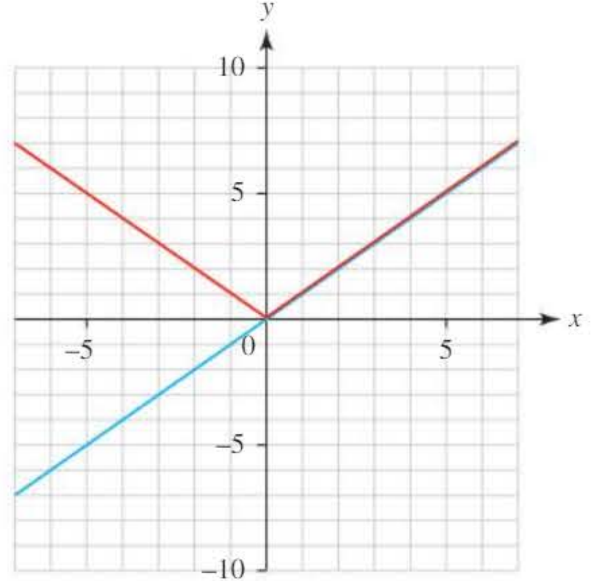
The diagram shows the graphs of (in blue) and (in red) drawn on the same axes. Notice how the negative portion of the line has been reflected upward to create the characteristic V-shape of the absolute value function.
Modulus Transformation Rule
When you carry out the reflection for the modulus function, any minimum turning point below the x-axis will be reflected into a maximum turning point above the x-axis. The x-coordinate stays the same, but the y-coordinate changes sign.
Worked example 3: Modulus of linear and quadratic functions
Worked Example: Linear and Quadratic Modulus
a) Sketch and for
The function is a straight line with gradient 2.
- x-intercept:
- y-intercept:
For , we reflect the negative part (where ) in the x-axis. The modulus graph crosses the axes at and .
b) Sketch and for
This is a positive quadratic curve (U-shaped).
- x-intercepts: and
- y-intercept:
For , we reflect the negative part (between the roots) in the x-axis. The modulus graph crosses the x-axis at and , and has a y-intercept at .
Worked example 4: General curve transformation
Worked Example: Modulus of a General Curve
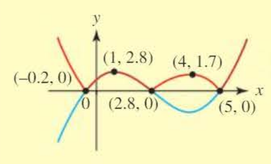
Given: A graph of showing points , , , , and .
Sketch
To create the modulus graph:
- Keep all parts of the graph that are above or on the x-axis
- Reflect the negative portion (around ) in the x-axis
- The minimum point becomes a maximum point
The red sections show the reflected portions, while the blue sections remain unchanged.
Worked example 5: Solving inequalities with transformations
Worked Example: Combined Transformations and Inequalities
The sketch shows part of the graph of .
a) Find the coordinates of the images of the points , and when is transformed into
Under the transformation :
- — negative y-coordinate becomes positive
- — negative y-coordinate becomes positive
- — positive y-coordinate stays the same
All negative parts of the graph are reflected in the x-axis.
b) Sketch the graph of and use it to solve
We reflect all negative parts of the graph upward. The horizontal line intersects at and .
Therefore, when .
c) Sketch the graph of and use it to estimate the solution to
For the reciprocal graph:
- The asymptote occurs approximately at (where )
- The point where becomes a vertical asymptote
- As becomes very large (either positive or negative), tends to zero
Since when , and from the graph, for (approximately), the solution is (approximately).
Key strategy for sketching transformations
To sketch a graph of or :
Step 1: If it has not been provided, sketch the graph of first. Identify all key features including roots, turning points, and intercepts.
Step 2: Consider the key features and transform them appropriately, clearly labeling the final graph with all important points, asymptotes, and coordinates.
Exam Tips
- Always check whether you're dealing with a reciprocal transformation or a modulus transformation
- For reciprocal graphs, pay special attention to vertical asymptotes at zeros of
- For modulus graphs, remember that only negative parts get reflected
- Label all transformed coordinates clearly, especially turning points
- When solving inequalities graphically, draw horizontal or vertical lines to find intersection points
- The sign of always matches the sign of
Remember!
Key Points to Remember:
-
Reciprocal graphs have vertical asymptotes at the zeros of the original function, and the sign of matches the sign of .
-
When , the original and reciprocal graphs intersect because .
-
Maximum points become minimum points (and vice versa) in reciprocal graphs, except when these points are at where they become asymptotes instead.
-
Modulus graphs reflect all negative portions of the original function upward across the x-axis, making all y-values positive or zero.
-
To sketch transformations efficiently, always start by sketching first if it's not provided, then systematically apply the transformation rules to key features.