Transformations Revision Notes for AQA A-Level Further Maths

Transformations

Introduction to matrix transformations

Matrices allow us to describe certain geometric transformations including rotations, reflections and enlargements. When we can represent a transformation using a matrix, we call it a linear transformation.

A point with coordinates $(x, y)$ can be represented by a position vector $\begin{pmatrix} x \\ y \end{pmatrix}$ . To transform this point, we apply a transformation matrix by pre-multiplying the vector. This means we multiply the vector by the transformation matrix, placing the matrix on the left side of the multiplication.

infoNote

Pre-multiplication is essential for transformations. The transformation matrix must always be on the left: $\mathbf{T}\mathbf{x}$ , not $\mathbf{x}\mathbf{T}$ . This ordering ensures the matrix multiplication is defined and produces the correct result.

Finding the image of a vector

To calculate where a vector moves to under a transformation, we use matrix multiplication. If we have a transformation matrix $\mathbf{T} = \begin{pmatrix} a & b \\ c & d \end{pmatrix}$ and want to find the image of vector $\begin{pmatrix} x \\ y \end{pmatrix}$ , we compute:

$\begin{pmatrix} x' \\ y' \end{pmatrix} = \begin{pmatrix} a & b \\ c & d \end{pmatrix}\begin{pmatrix} x \\ y \end{pmatrix}$

The result $\begin{pmatrix} x' \\ y' \end{pmatrix}$ represents the new position after the transformation.

lightbulbExample

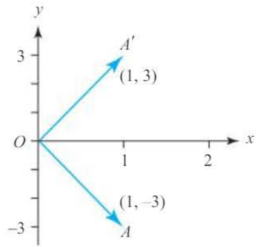
Worked Example: Reflection in the x-axis

Consider finding the image of point $A(1, -3)$ under the transformation $\mathbf{T} = \begin{pmatrix} 1 & 0 \\ 0 & -1 \end{pmatrix}$ .

Step 1: Represent point $A$ as the vector $\begin{pmatrix} 1 \\ -3 \end{pmatrix}$

Step 2: Multiply by $\mathbf{T}$ :

$\begin{pmatrix} x' \\ y' \end{pmatrix} = \begin{pmatrix} 1 & 0 \\ 0 & -1 \end{pmatrix}\begin{pmatrix} 1 \\ -3 \end{pmatrix} = \begin{pmatrix} 1 \\ 3 \end{pmatrix}$

Result: This is a reflection in the x-axis. The point moves from $(1, -3)$ to $(1, 3)$ .

Standard 2D transformation matrices

Reflection matrices

Different matrices produce reflections in different lines. You need to memorise these standard reflection matrices:

Reflection in the x-axis: $\begin{pmatrix} 1 & 0 \\ 0 & -1 \end{pmatrix}$

Reflection in the y-axis: $\begin{pmatrix} -1 & 0 \\ 0 & 1 \end{pmatrix}$

Reflection in the line $y = x$ : $\begin{pmatrix} 0 & 1 \\ 1 & 0 \end{pmatrix}$

Reflection in the line $y = -x$ : $\begin{pmatrix} 0 & -1 \\ -1 & 0 \end{pmatrix}$

infoNote

Memory Aid for Reflection in $y=x$ :

For the $y=x$ reflection, notice that the off-diagonal positions swap to give $\begin{pmatrix} 0 & 1 \\ 1 & 0 \end{pmatrix}$ . This swapping of positions reflects the swapping of $x$ and $y$ coordinates.

Rotation matrices

For an anticlockwise rotation by angle $\theta$ about the origin, we use the matrix:

$\begin{pmatrix} \cos\theta & -\sin\theta \\ \sin\theta & \cos\theta \end{pmatrix}$

Note that positive angles always give anticlockwise rotations. The pattern here is helpful to remember: cosine appears on the leading diagonal, sine appears on the other diagonal with a negative sign in the top-right position.

chatImportant

Rotation Matrix Pattern:

Remember: "Cos on diagonal, sin swapped with negative"

$\begin{pmatrix} \cos & -\sin \\ \sin & \cos \end{pmatrix}$

This pattern makes it easier to recall the correct positions and signs when writing rotation matrices.

Stretch matrices

A stretch changes distances in one direction only. The stretch is parallel to one of the coordinate axes.

Stretch with scale factor $k$ parallel to the x-axis: $\begin{pmatrix} k & 0 \\ 0 & 1 \end{pmatrix}$

This multiplies x-coordinates by $k$ while leaving y-coordinates unchanged.

Stretch with scale factor $k$ parallel to the y-axis: $\begin{pmatrix} 1 & 0 \\ 0 & k \end{pmatrix}$

This multiplies y-coordinates by $k$ while leaving x-coordinates unchanged.

infoNote

Memory Aid for Stretches:

The scale factor $k$ on the diagonal stretches that axis: $k$ in the top-left position stretches the x-direction, while $k$ in the bottom-right position stretches the y-direction.

Enlargement matrices

An enlargement with scale factor $k$ and centre at the origin changes distances equally in all directions:

$\begin{pmatrix} k & 0 \\ 0 & k \end{pmatrix}$

This multiplies both coordinates by $k$ , scaling the entire figure.

The identity matrix

The identity matrix is a special matrix that leaves all points unchanged:

$\mathbf{I} = \begin{pmatrix} 1 & 0 \\ 0 & 1 \end{pmatrix}$

It has the important property that for any $2 \times 2$ matrix $\mathbf{A}$ :

$\mathbf{AI} = \mathbf{IA} = \mathbf{A}$

This is similar to how multiplying a number by 1 leaves it unchanged.

Finding transformation matrices

When a transformation is described geometrically but you need to find its matrix, consider what happens to the basis vectors $\begin{pmatrix} 1 \\ 0 \end{pmatrix}$ and $\begin{pmatrix} 0 \\ 1 \end{pmatrix}$ .

The key principle is:

The matrix $\begin{pmatrix} a & b \\ c & d \end{pmatrix}$ describes a transformation that maps:

$\begin{pmatrix} 1 \\ 0 \end{pmatrix}$ to $\begin{pmatrix} a \\ c \end{pmatrix}$
$\begin{pmatrix} 0 \\ 1 \end{pmatrix}$ to $\begin{pmatrix} b \\ d \end{pmatrix}$

This means the first column of the matrix shows where $\begin{pmatrix} 1 \\ 0 \end{pmatrix}$ moves to, and the second column shows where $\begin{pmatrix} 0 \\ 1 \end{pmatrix}$ moves to.

chatImportant

The Basis Vector Method:

The columns of a transformation matrix represent the images of the basis vectors:

First column = image of $\begin{pmatrix} 1 \\ 0 \end{pmatrix}$
Second column = image of $\begin{pmatrix} 0 \\ 1 \end{pmatrix}$

This is the key to finding any transformation matrix from a geometric description.

lightbulbExample

Worked Example: Finding a Rotation Matrix

Find the $2 \times 2$ matrix that represents a rotation of $90°$ anticlockwise about the origin.

Solution:

Let the matrix be $\begin{pmatrix} a & b \\ c & d \end{pmatrix}$ .

Step 1: Choose the two basis vectors and determine their images after a $90°$ anticlockwise rotation:

$(1, 0)$ moves to $(0, 1)$
$(0, 1)$ moves to $(-1, 0)$

Step 2: Apply the matrix equation for the first basis vector: $\begin{pmatrix} a & b \\ c & d \end{pmatrix}\begin{pmatrix} 1 \\ 0 \end{pmatrix} = \begin{pmatrix} 0 \\ 1 \end{pmatrix}$

This gives us $a = 0$ and $c = 1$ .

Step 3: Apply the matrix equation for the second basis vector: $\begin{pmatrix} a & b \\ c & d \end{pmatrix}\begin{pmatrix} 0 \\ 1 \end{pmatrix} = \begin{pmatrix} -1 \\ 0 \end{pmatrix}$

This gives us $b = -1$ and $d = 0$ .

Result: The transformation matrix is: $\begin{pmatrix} 0 & -1 \\ 1 & 0 \end{pmatrix}$

lightbulbExample

Worked Example: Finding a 60° Rotation Matrix

Find the matrix representing a $60°$ anticlockwise rotation about the origin.

Solution:

Using the basis vectors:

$\begin{pmatrix} 1 \\ 0 \end{pmatrix}$ maps to $\begin{pmatrix} \cos 60° \\ \sin 60° \end{pmatrix}$
$\begin{pmatrix} 0 \\ 1 \end{pmatrix}$ maps to $\begin{pmatrix} -\sin 60° \\ \cos 60° \end{pmatrix}$

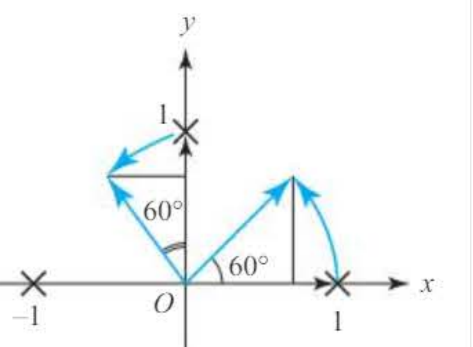
Result: The transformation matrix is: $\begin{pmatrix} \cos 60° & -\sin 60° \\ \sin 60° & \cos 60° \end{pmatrix} = \begin{pmatrix} \frac{1}{2} & -\frac{\sqrt{3}}{2} \\ \frac{\sqrt{3}}{2} & \frac{1}{2} \end{pmatrix}$

Transforming multiple points simultaneously

Transformations can be applied to several points at once by forming a matrix from their position vectors. Each column represents one point.

lightbulbExample

Worked Example: Enlargement of Multiple Points

Find the image of the points $(2, -1)$ , $(-4, 5)$ and $(-3, 0)$ under the transformation described by $\begin{pmatrix} 2 & 0 \\ 0 & 2 \end{pmatrix}$ . Describe the transformation geometrically.

Solution:

Form a matrix with the position vectors as columns:

$\begin{pmatrix} 2 & 0 \\ 0 & 2 \end{pmatrix}\begin{pmatrix} 2 & -4 & -3 \\ -1 & 5 & 0 \end{pmatrix} = \begin{pmatrix} 4 & -8 & -6 \\ -2 & 10 & 0 \end{pmatrix}$

Result: The image points are $(4, -2)$ , $(-8, 10)$ and $(-6, 0)$ .

This is an enlargement of scale factor 2, centre the origin. Each coordinate is multiplied by 2.

Combined transformations

When we apply one transformation followed by another, we can represent the combined effect using matrix multiplication. However, the order of matrices is important.

If transformation $\mathbf{A}$ is followed by transformation $\mathbf{B}$ , then $\mathbf{BA}$ represents the combined transformation.

Notice the order: to apply transformation $\mathbf{A}$ to a vector first, you multiply by $\mathbf{A}$ . Then to apply $\mathbf{B}$ , you multiply the result by $\mathbf{B}$ . This gives $\mathbf{B}(\mathbf{A}\mathbf{x}) = (\mathbf{BA})\mathbf{x}$ , hence $\mathbf{BA}$ .

chatImportant

Remember the Order of Transformations:

$\mathbf{BA}$ means apply $\mathbf{A}$ first, then $\mathbf{B}$ . The order is read right to left.

This is like function composition: if you write $f(g(x))$ , you apply $g$ first, then $f$ . Similarly, $\mathbf{BA}\mathbf{x}$ means apply $\mathbf{A}$ first, then $\mathbf{B}$ .

Memory Aid: ROT-ATION = Remember Order of Transformations - Apply from right to left.

lightbulbExample

Worked Example: Rotation Followed by Reflection

Find the single matrix that represents a rotation of $270°$ anticlockwise followed by a reflection in the y-axis.

Solution:

Step 1: Identify the rotation matrix.

For rotation of $270°$ anticlockwise:

$\begin{pmatrix} 1 \\ 0 \end{pmatrix}$ is transformed to $\begin{pmatrix} 0 \\ -1 \end{pmatrix}$
$\begin{pmatrix} 0 \\ 1 \end{pmatrix}$ is transformed to $\begin{pmatrix} 1 \\ 0 \end{pmatrix}$

Therefore $\mathbf{A} = \begin{pmatrix} 0 & 1 \\ -1 & 0 \end{pmatrix}$

Step 2: Identify the reflection matrix.

For reflection in the y-axis:

$\begin{pmatrix} 1 \\ 0 \end{pmatrix}$ is transformed to $\begin{pmatrix} -1 \\ 0 \end{pmatrix}$
$\begin{pmatrix} 0 \\ 1 \end{pmatrix}$ is transformed to $\begin{pmatrix} 0 \\ 1 \end{pmatrix}$

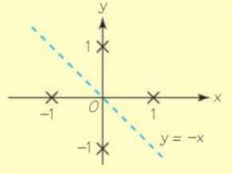
Therefore $\mathbf{B} = \begin{pmatrix} -1 & 0 \\ 0 & 1 \end{pmatrix}$

Step 3: Calculate the combined transformation $\mathbf{BA}$ :

$\mathbf{BA} = \begin{pmatrix} -1 & 0 \\ 0 & 1 \end{pmatrix}\begin{pmatrix} 0 & 1 \\ -1 & 0 \end{pmatrix} = \begin{pmatrix} 0 & -1 \\ -1 & 0 \end{pmatrix}$

Result: This is a reflection in the line $y = -x$ .

3D transformations

We use $3 \times 3$ matrices to represent transformations in three-dimensional space. Points in 3D have position vectors $\begin{pmatrix} x \\ y \\ z \end{pmatrix}$ .

3D reflection matrices

To reflect in a coordinate plane, we change the sign of the coordinate perpendicular to that plane.

Reflection in the plane $x = 0$ (the yz-plane): $\begin{pmatrix} -1 & 0 & 0 \\ 0 & 1 & 0 \\ 0 & 0 & 1 \end{pmatrix}$

Reflection in the plane $y = 0$ (the xz-plane): $\begin{pmatrix} 1 & 0 & 0 \\ 0 & -1 & 0 \\ 0 & 0 & 1 \end{pmatrix}$

Reflection in the plane $z = 0$ (the xy-plane): $\begin{pmatrix} 1 & 0 & 0 \\ 0 & 1 & 0 \\ 0 & 0 & -1 \end{pmatrix}$

3D rotation matrices

When rotating around a coordinate axis, the coordinate along that axis stays unchanged. This creates a $2 \times 2$ rotation pattern within the $3 \times 3$ matrix.

infoNote

Pattern for 3D Rotations:

The axis you rotate around stays still. That coordinate doesn't change, so you see the standard 2D rotation matrix in the other two coordinates. The unchanged coordinate has a 1 in its position on the diagonal and zeros elsewhere.

Rotation around the x-axis by angle $\theta$ anticlockwise: $\begin{pmatrix} 1 & 0 & 0 \\ 0 & \cos\theta & -\sin\theta \\ 0 & \sin\theta & \cos\theta \end{pmatrix}$

The x-coordinate doesn't change, and we see the standard 2D rotation in the yz-coordinates.

Rotation around the y-axis by angle $\theta$ anticlockwise: $\begin{pmatrix} \cos\theta & 0 & \sin\theta \\ 0 & 1 & 0 \\ -\sin\theta & 0 & \cos\theta \end{pmatrix}$

Rotation around the z-axis by angle $\theta$ anticlockwise: $\begin{pmatrix} \cos\theta & -\sin\theta & 0 \\ \sin\theta & \cos\theta & 0 \\ 0 & 0 & 1 \end{pmatrix}$

The z-coordinate doesn't change, and we see the standard 2D rotation in the xy-coordinates.

lightbulbExample

Worked Example: 3D Rotation Around x-axis

Find the $3 \times 3$ matrix $\mathbf{T}$ that represents a rotation of $45°$ anticlockwise around the x-axis, and find the image of point $P(1, 4, -2)$ under $\mathbf{T}$ .

Solution:

Step 1: Write the rotation matrix using the formula:

$\mathbf{T} = \begin{pmatrix} 1 & 0 & 0 \\ 0 & \cos 45° & -\sin 45° \\ 0 & \sin 45° & \cos 45° \end{pmatrix} = \begin{pmatrix} 1 & 0 & 0 \\ 0 & \frac{\sqrt{2}}{2} & -\frac{\sqrt{2}}{2} \\ 0 & \frac{\sqrt{2}}{2} & \frac{\sqrt{2}}{2} \end{pmatrix}$

Step 2: Pre-multiply the vector representing point $P$ by matrix $\mathbf{T}$ :

$P' = \begin{pmatrix} 1 & 0 & 0 \\ 0 & \frac{\sqrt{2}}{2} & -\frac{\sqrt{2}}{2} \\ 0 & \frac{\sqrt{2}}{2} & \frac{\sqrt{2}}{2} \end{pmatrix}\begin{pmatrix} 1 \\ 4 \\ -2 \end{pmatrix}$

$= \begin{pmatrix} 1 \\ \frac{\sqrt{2}}{2}(4) + \frac{\sqrt{2}}{2}(2) \\ \frac{\sqrt{2}}{2}(4) - \frac{\sqrt{2}}{2}(2) \end{pmatrix}$

$= \begin{pmatrix} 1 \\ 2\sqrt{2} + \sqrt{2} \\ 2\sqrt{2} - \sqrt{2} \end{pmatrix} = \begin{pmatrix} 1 \\ 3\sqrt{2} \\ \sqrt{2} \end{pmatrix}$

Result: The image point is $(1, 3\sqrt{2}, \sqrt{2})$ .

Invariant points

An invariant point is a point that remains unchanged when a transformation is applied to it. If we have transformation matrix $\mathbf{T}$ and position vector $\mathbf{x}$ , then:

If $\mathbf{Tx} = \mathbf{x}$ , then $\mathbf{x}$ represents an invariant point.

For any linear transformation, the origin $(0, 0)$ is always an invariant point, because:

$\mathbf{T}\begin{pmatrix} 0 \\ 0 \end{pmatrix} = \begin{pmatrix} 0 \\ 0 \end{pmatrix}$

infoNote

Memory Aid: " $\mathbf{T}$ of $\mathbf{x}$ equals $\mathbf{x}$ " - the point stays the same under the transformation.

Method for finding invariant points

To find invariant points:

Write a general vector $\begin{pmatrix} x \\ y \end{pmatrix}$ to represent the invariant point
Pre-multiply by the transformation matrix to form simultaneous equations
Solve the equations to find either a specific point or a line of invariant points
If finding invariant lines, equate coefficients to determine the equation

lightbulbExample

Worked Example: Finding an Invariant Point

Find any invariant points under the transformation given by $\begin{pmatrix} 3 & 1 \\ -1 & 2 \end{pmatrix}$ .

Solution:

Step 1: Let $\begin{pmatrix} x \\ y \end{pmatrix}$ be an invariant point.

Then: $\begin{pmatrix} 3 & 1 \\ -1 & 2 \end{pmatrix}\begin{pmatrix} x \\ y \end{pmatrix} = \begin{pmatrix} x \\ y \end{pmatrix}$

Step 2: This gives: $3x + y = x$ $-x + 2y = y$

Step 3: Simplifying: $2x + y = 0$ $-x + y = 0$

Step 4: From the second equation: $y = x$

Substituting into the first equation: $2x + x = 0$ , so $3x = 0$ and $x = 0$ .

Therefore $y = 0$ .

Result: The only invariant point is $(0, 0)$ .

Lines of invariant points

Some transformations have a line of invariant points where every point on the line maps to itself under the transformation.

For example, consider a reflection in the line $y = x$ . Every point on this line is unchanged by the reflection, so $y = x$ is a line of invariant points.

lightbulbExample

Worked Example: Finding a Line of Invariant Points

Find the invariant points under the transformation given by $\begin{pmatrix} 2 & 3 \\ -1 & -2 \end{pmatrix}$ .

Solution:

Step 1: Let $\begin{pmatrix} x \\ y \end{pmatrix}$ be an invariant point.

Then: $\begin{pmatrix} 2 & 3 \\ -1 & -2 \end{pmatrix}\begin{pmatrix} x \\ y \end{pmatrix} = \begin{pmatrix} x \\ y \end{pmatrix}$

Step 2: This gives: $2x + 3y = x \Rightarrow x = -3y$ $-x - 2y = y \Rightarrow x = -3y$

Step 3: Both equations simplify to the same result: $x = -3y$ .

Result: This represents a line through the origin. Any point of the form $(−3y, y)$ is invariant, so there is a line of invariant points given by $x = -3y$ .

Invariant lines

An invariant line is different from a line of invariant points. For an invariant line, every point on the line maps to another point on the same line (but not necessarily to itself).

chatImportant

Key Distinction:

Line of invariant points: Every point on the line maps to itself
Invariant line: Every point on the line maps to another point on the same line

For example, consider a rotation of $180°$ around the origin. The origin $(0, 0)$ is invariant, but if you take any line through the origin, every point on that line rotates to a different point on the same line. These are invariant lines, not lines of invariant points.

To find equations of invariant lines, use $y = mx + c$ to represent the general form, then use the transformation to find possible values of $m$ and $c$ .

lightbulbExample

Worked Example: Finding Invariant Lines

Find the equations of the invariant lines of the transformation given by $\begin{pmatrix} 1 & 1 \\ 0 & 3 \end{pmatrix}$ .

Solution:

Step 1: Write the general point on a line as $\begin{pmatrix} x \\ mx + c \end{pmatrix}$ where the line has equation $y = mx + c$ .

Step 2: Apply the transformation: $\begin{pmatrix} 1 & 1 \\ 0 & 3 \end{pmatrix}\begin{pmatrix} x \\ mx + c \end{pmatrix} = \begin{pmatrix} x' \\ y' \end{pmatrix}$

This gives: $x' = x + mx + c$ $y' = 3(mx + c)$

Step 3: For the image to lie on the same line, we need $y' = mx' + c$ .

Substituting: $3(mx + c) = m(x + mx + c) + c$

Step 4: Expanding: $3mx + 3c = mx + m^2x + mc + c$

Step 5: Collecting terms in $x$ : $(3m - m - m^2)x + 3c - mc - c = 0$

For this to be true for all values of $x$ , we need:

Coefficient of $x$ : $3m - m - m^2 = 0$ , which gives $2m - m^2 = 0$ , so $m(2 - m) = 0$
Constant term: $2c - mc = 0$

Step 6: From the coefficient equation: $m = 0$ or $m = 2$ .

When $m = 0$ : The constant term equation gives $2c = 0$ , so $c = 0$ . This means $y = 0$ is an invariant line.

When $m = 2$ : The constant term equation gives $2c - 2c = 0$ , which is satisfied for any value of $c$ . This means $y = 2x + c$ is an invariant line for any value of $c$ .

Result: The invariant lines are $y = 0$ and $y = 2x + c$ (for any constant $c$ ).

bookmarkSummary

Key Points to Remember:

Always pre-multiply: To transform a vector, multiply it by the transformation matrix on the left: $\mathbf{Tx}$
Standard matrices: Memorise the reflection, rotation, stretch and enlargement matrices
Basis vector method: The columns of a transformation matrix show where $\begin{pmatrix} 1 \\ 0 \end{pmatrix}$ and $\begin{pmatrix} 0 \\ 1 \end{pmatrix}$ move to
Order matters for combinations: $\mathbf{BA}$ means apply $\mathbf{A}$ first, then $\mathbf{B}$ - the order is read right to left
Origin is always invariant: For any linear transformation, $(0, 0)$ always maps to itself
Invariant points vs invariant lines: Points on a line of invariant points map to themselves; points on an invariant line map to other points on the same line

Transformations (AQA A-Level Further Maths): Revision Notes