Euler’s Method (AQA A-Level Further Maths): Revision Notes

Euler's Method

Introduction

Most first-order differential equations cannot be solved using standard calculus and algebra techniques. When this happens, you need to use numerical methods to find approximate solutions. Euler's method is one such numerical technique that allows you to estimate successive points on a solution curve.

What is Euler's method?

Euler's method is a numerical technique for approximating solutions to differential equations of the form:

$\frac{dy}{dx} = f(x, y)$

where you know one starting point $(x_0, y_0)$ that lies on the solution curve.

The method is named after Swiss mathematician Leonhard Euler (1707-1783).

The basic principle

Euler's method works by using the gradient of the tangent line at a known point to estimate the next point along the solution curve. Since $\frac{dy}{dx} = f(x_0, y_0)$ at the point $(x_0, y_0)$, the value of $f(x_0, y_0)$ represents the gradient of the tangent to the solution curve at that point.

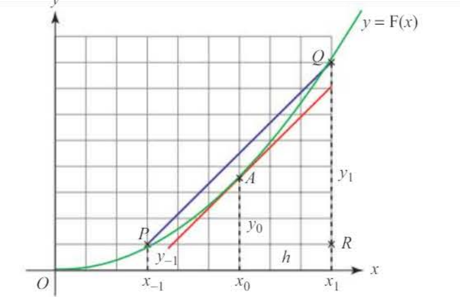
On a straight line, the change in $y$ equals the change in $x$ times the gradient. If $x$ increases by a small amount $h$ (called the step length), then $y$ increases by approximately $h \times f(x_0, y_0)$.

The Euler formula

The iterative process of Euler's method can be expressed using a simple formula that generates successive approximations along the solution curve:

This process can be repeated to generate successive approximations: $(x_1, y_1)$, $(x_2, y_2)$, $(x_3, y_3)$, and so on, which lie approximately on the solution curve.

Accuracy considerations

Understanding the factors that affect accuracy is crucial for applying Euler's method effectively in practice.

Worked example 1: Basic Euler's method

Worked example 2: Euler's method with complex function

The improved Euler method

The improved Euler method provides better accuracy by using the average of the gradients at the initial point and the end point of each step.

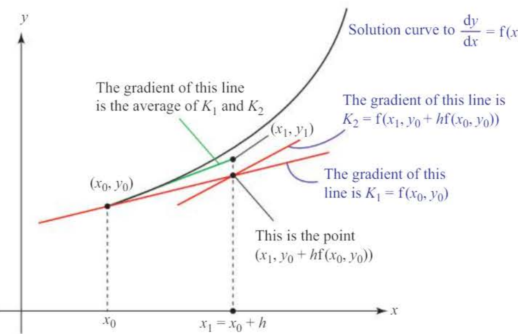
How it works

Let $A$ be the point $(x_0, y_0)$ and $B$ be the point $(x_1, y_1)$.

Using basic Euler's method: $x_1 = x_0 + h$ and $y_1 = y_0 + hf(x_0, y_0)$

The improved method calculates two gradients:

• $k_1 = hf(x_0, y_0)$ - the gradient at point $A$
• $k_2 = hf(x_0 + h, y_0 + k_1)$ - the gradient at point $B$

Then the improved estimate is:

$y_1 = y_0 + \frac{1}{2}(k_1 + k_2)$

Worked example 3: Improved Euler method

The midpoint method

The midpoint method is an alternative improved Euler method. It compares the gradient of the chord $PQ$ on a curve $F(x, y)$ with the gradient of the curve $f(x, y)$ at the midpoint of the chord.

The formula

Let $P$ be $(x_{-1}, y_{-1})$ and let $Q$ be $(x_1, y_1)$, with $x_0 - x_{-1} = x_1 - x_0 = h$.

The gradient of the chord $PQ$ is: $\frac{QR}{PR} = \frac{y_1 - y_{-1}}{x_1 - x_{-1}} = \frac{y_1 - y_{-1}}{2h}$

This gradient approximates the gradient of the curve at the midpoint $A$, so: $f(x_0, y_0) = \frac{y_1 - y_{-1}}{2h}$

Rearranging gives:

Worked example 4: Midpoint method

Problem-solving strategy

When solving differential equations numerically using Euler's method, follow this systematic approach to ensure accuracy and completeness:

Step 1: Identify the differentiated function $f(x, y)$, a starting point $(x_0, y_0)$, and a suitable step value $h$.

Step 2: Calculate $y_1 = y_0 + hf(x_0, y_0)$.

Step 3: Continue using $y_{r+1} = y_r + hf(x_r, y_r)$ until the desired endpoint is reached.

Step 4: Answer the question in context (including units where appropriate).

Using spreadsheets

For questions requiring many iterations, use a spreadsheet, graphical calculator, or computer software. This removes the tedious arithmetic and reduces calculation errors.

Exam tips

Remember!