Factors Leading to a Change in Supply (Edexcel A-Level Business): Revision Notes
Factors Leading to a Change in Supply
Understanding supply shifts
Supply represents the quantity of a good or service that producers are willing and able to make available to the market at any given price level. The relationship between price and quantity supplied is typically positive - as prices rise, producers are incentivised to supply more because profitability increases.
It is crucial to distinguish between two types of changes in supply:
- Movement along the supply curve - caused solely by price changes. When the price of a product rises or falls, there is a movement up or down the existing supply curve.
- Shift of the supply curve - caused by changes in factors other than price. These shifts represent a change in the quantity supplied at every price level.
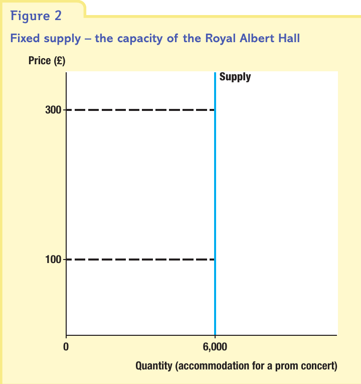
The supply curve is typically upward-sloping from left to right, showing the positive relationship between price and quantity supplied. However, understanding what causes the entire curve to shift position is essential for analysing real-world market changes.
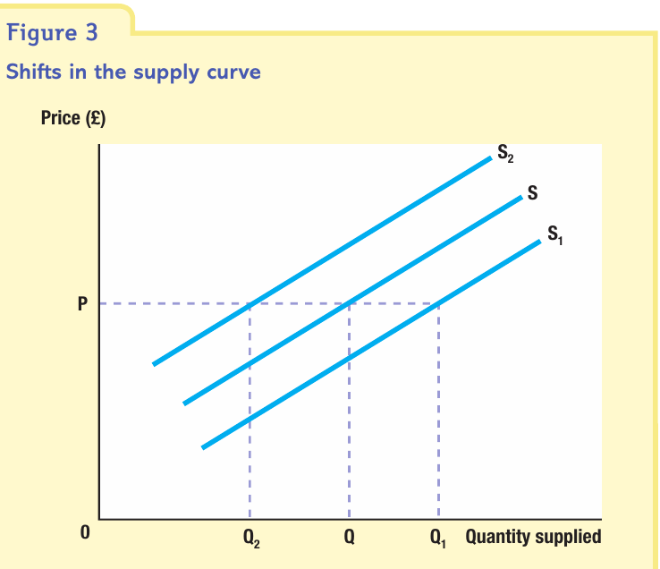
Figure 3 above illustrates how the supply curve shifts. The original supply curve is marked as S. When supply increases (shift to the right to S₁), more is supplied at every price level - at price P, quantity increases from Q to Q₁. When supply decreases (shift to the left to S₂), less is supplied at every price level - at price P, quantity falls from Q to Q₂.
Five key factors that shift the supply curve
Changes in the costs of production
Production costs are fundamental determinants of supply. These costs include wages, raw materials, energy, rent, and machinery expenses. When production costs change, profitability changes, which directly affects how much producers are willing to supply.
Rising costs impact: If production costs increase, profit margins are squeezed. Producers respond by reducing the quantity they are willing to supply at each price level. This causes the supply curve to shift left (from S to S₂).
Real-World Example: Tata Chemicals Closure
In 2013, Tata Chemicals closed its soda ash factory in Northwich after 139 years of operation. The closure resulted from rising gas prices which made production unprofitable, demonstrating how cost increases can eliminate supply entirely.
Falling costs impact: Conversely, when production costs fall, profit margins improve. Producers are incentivised to increase output because production is more profitable. This shifts the supply curve right (from S to S₁), meaning more is supplied at every price level.
Resource availability also plays a critical role. Shortages in factors of production - such as skilled labour, raw materials, or capital equipment - make it difficult for producers to supply markets effectively. Between 2013 and 2014, the UK experienced significant skills shortages across approximately 40 different sectors. Engineering skills (electrical, civil, software, mechanical), IT professionals (programmers, developers, coders), NHS medical staff, and teachers were all in short supply. These labour shortages constrained economic growth by limiting the ability of businesses to increase production and supply.
Introduction of new technology
Technological advancement typically increases supply by improving production efficiency and reducing costs per unit. When businesses adopt new technology, they can produce more output with the same resources, or maintain output levels while using fewer resources.
Effect on supply curve: The introduction of new technology shifts the supply curve to the right (from S to S₁). At any given price P, the quantity supplied increases from Q to Q₁ because production is now more efficient and cost-effective.
Real-World Application: UK Manufacturing Revival
Britain's manufacturing sector has demonstrated this effect clearly. Advanced technology adoption in car manufacturing and aerospace has improved both products and production processes. The strength of these technology-intensive industries helped revive UK manufacturing after 2008, following three decades of decline. This shows how technological progress can reverse negative supply trends and strengthen entire economic sectors.

Agricultural technology provides another example. The development of "farmbots" - robots designed for farming tasks - aims to increase efficiency in agriculture. These machines can perform complex tasks that traditional large-scale machinery cannot accomplish, such as precision weeding around individual lettuce plants or pruning vines in vineyards. While widespread commercial adoption may take decades, such technological innovations have the potential to significantly increase agricultural supply when they become economically viable.
Indirect taxes
Indirect taxes are taxes levied on spending rather than on income. Value Added Tax (VAT) and excise duties on products like petrol, alcohol, and tobacco are common examples in the UK.
Effect on supply: Indirect taxes represent an additional cost to businesses. When the government imposes a new indirect tax or increases an existing one, the supply curve shifts left (from S to S₂). This is because producers' costs have increased, reducing the quantity they are willing to supply at each price level.
Tax reduction: If the government reduces or removes an indirect tax, production costs fall. The supply curve shifts right (from S to S₁), indicating that producers are willing to supply more at every price level.
Real-World Example: The 2011 VAT Increase
In January 2011, the UK government raised VAT from 17.5% to 20%. This 2.5 percentage point increase acted as a cost increase for businesses and a disincentive to production. Many economists argued that this tax rise would prolong the recession by discouraging supply.
Tax burden sharing: Following the imposition of an indirect tax, the financial burden is typically shared between consumers and producers. The proportion each party bears depends largely on the price elasticity of demand. When demand is relatively inelastic (consumers are not very responsive to price changes), consumers bear a larger share of the tax burden through higher prices. When demand is elastic, producers absorb more of the tax through reduced profit margins.
Government subsidies
A subsidy is a financial grant given by the government to producers, typically to encourage production of particular goods or services that are considered economically or socially beneficial.
Effect on supply: Subsidies effectively reduce production costs for businesses. When the government grants a subsidy, the supply curve shifts right (from S to S₁). Producers are willing to supply more at every price level because their costs have been reduced, improving profitability.
Real-World Example: UK Renewable Energy Subsidies
In 2014, the UK government announced $300 million in subsidies for the renewable energy industry. This formed part of Britain's strategy to cut greenhouse gas emissions by 80% from 1990s levels by 2050. The subsidies were awarded to low-carbon electricity projects through competitive auctions and distributed on 15-year contracts. By reducing the costs of renewable energy production, these subsidies aimed to increase the supply of clean energy and accelerate the transition away from fossil fuels.
Strategic use: Governments use subsidies strategically to:
- Encourage production of merit goods (goods that society benefits from)
- Support declining industries during transition periods
- Promote environmental objectives
- Maintain supply of essential goods and services
- Encourage innovation and development in emerging sectors
External shocks
External shocks are unexpected events or factors beyond the direct control of businesses that significantly impact supply. These can cause sudden and sometimes dramatic shifts in supply curves.
World events: Global political and economic events can disrupt supply chains and production capabilities. The Middle East oil supply provides a clear example - political instability in this region regularly threatens oil supplies because a significant proportion of global oil comes from these countries. When tensions escalate, the supply of oil contracts, shifting the supply curve left and driving prices up.
The 2008 global financial crisis created a "credit crunch" where businesses found it difficult or impossible to borrow money for trading and investment. Many firms collapsed, while others could not expand. This external shock severely reduced supply across numerous sectors of the economy.
Weather conditions: Agricultural supply is particularly vulnerable to weather variations. Favourable growing conditions lead to bumper harvests and increased supply, shifting the supply curve right. Conversely, droughts, floods, or other adverse weather reduce crop yields, shifting supply left and creating shortages.
Real-World Example: 2014 European Wheat Harvest
In 2014, Europe and the Black Sea region experienced ideal growing conditions, resulting in bumper wheat crops. The increase in global wheat supply caused prices to fall. This demonstrates how weather can cause significant year-to-year supply fluctuations in agricultural markets.
Extreme weather events like snowstorms can also disrupt supply in the short term by hampering distribution networks. Closed roads, railway lines, and airports prevent goods from reaching markets, temporarily reducing available supply even though production may be unaffected.
Government policies: Government economic policy decisions can impact supply significantly. If the Bank of England increases interest rates (perhaps to control inflation), businesses with debt face higher costs. Additionally, higher interest rates discourage borrowing for investment, which can constrain future supply growth.
Government legislation also affects supply. Laws designed to increase market competition typically increase supply as new firms enter the market. Conversely, restrictive regulations can reduce supply by making production more costly or difficult.
Price of related goods: In some markets, producers can switch between supplying different products. When this is possible, changes in the relative prices of these goods affect supply decisions.
Real-World Example: Farmer Crop Switching
An arable farmer primarily growing potatoes might observe rising prices for carrots and parsnips. If these price increases are substantial, the farmer might decide to allocate more land to carrots and parsnips in the next growing season, reducing potato supply. This demonstrates how the supply of one good can be influenced by price changes in related goods that producers could alternatively supply.
Fixed supply in special cases
In certain circumstances, supply may be completely fixed regardless of price changes. When this occurs, the supply curve becomes vertical, indicating that quantity supplied cannot increase even when prices rise significantly.
The capacity of venues such as concert halls, theatres, and sports stadiums provides a clear example. The Royal Albert Hall can accommodate approximately 6,000 people for the Proms concerts. Even if ticket prices increased from $100 to $300, no additional seats could be supplied because the venue's physical capacity is fixed. The supply curve is therefore perfectly vertical at 6,000, showing zero responsiveness to price changes.
This concept is important when analysing markets where supply cannot be expanded in the relevant time period, either due to physical constraints or because production processes are lengthy and inflexible.
Short-term versus long-term supply considerations
The time horizon significantly affects supply responsiveness. This distinction is valuable when evaluating supply-side changes:
Short-term constraints: In the short term, many firms cannot easily increase supply even when market conditions are favourable. Farmers cannot increase crop supply until the next growing season. Manufacturers operating at full capacity need time to build additional production facilities. These short-term supply limitations mean quantity supplied may be relatively fixed or slow to respond to changes.
Long-term flexibility: Over longer time periods, supply becomes more flexible and responsive. Firms can adapt to changed market conditions by investing in additional capacity, hiring more workers, adopting new technology, or entering new markets. This means supply curves tend to be more elastic (responsive) in the long term than in the short term.
Application: UK housing supply
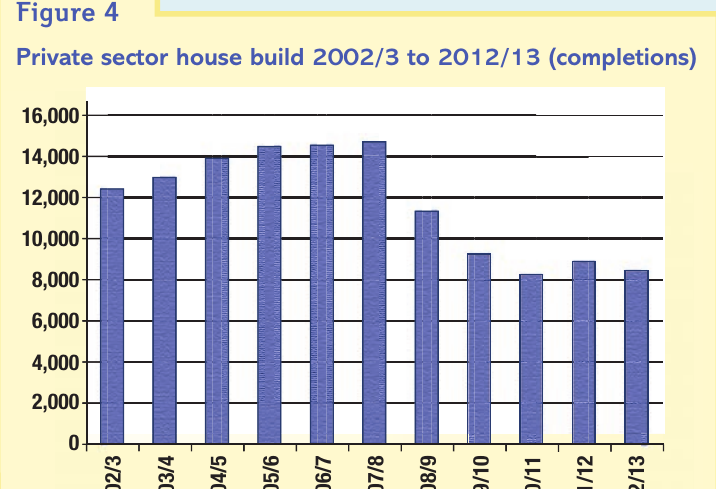

The UK housing market illustrates several supply factors in practice. Figure 4 shows that private sector house building peaked in 2007/8 at nearly 15,000 completions, then fell sharply following the 2008 financial crisis. By 2009/10, completions had dropped to around 9,000, where they remained through 2012/13.
Multiple factors contributed to this supply reduction:
- Financial crisis (external shock) - the credit crunch made it difficult for construction companies to borrow funds for development
- Rising costs - land prices and construction costs increased, squeezing profit margins
- Reduced subsidies - government support for housing construction declined
- Planning regulations - restrictive planning laws limited where and how much could be built
Despite rising house prices (indicating strong demand), supply remained constrained. This demonstrates that supply cannot always respond quickly to market signals, particularly when multiple negative factors combine.
Remember!
Key Points to Remember:
-
Supply shifts versus movements: Price changes cause movements along the supply curve, while changes in other factors shift the entire curve's position.
-
Five key factors shift supply: Changes in production costs, new technology, indirect taxes, government subsidies, and external shocks all shift the supply curve left (decrease) or right (increase).
-
Cost changes and technology have opposite effects: Rising costs shift supply left (decrease), falling costs shift supply right (increase). New technology shifts supply right by reducing per-unit costs.
-
Government can influence supply: Through indirect taxes (shift left), subsidies (shift right), interest rates, and legislation. These policy tools allow governments to encourage or discourage supply of particular goods.
-
External shocks are unpredictable: World events, weather conditions, and unexpected crises can cause sudden supply disruptions. These are particularly important in markets like oil (affected by political instability) and agriculture (affected by weather).
-
Time matters for supply analysis: Supply is typically more constrained in the short term due to fixed capacity and production lead times, but becomes more flexible in the long term as firms can invest and adapt.