Amphibian Phylogeny (VCE SSCE Biology): Revision Notes

Amphibian Phylogeny

Introduction to phylogenetic analysis

Scientists can work out how closely different species are related using several methods. One powerful approach involves genome sequencing, where researchers compare DNA and amino acid sequences between species. By examining the similarities and differences in genetic material, we can construct phylogenetic trees that visually show potential evolutionary relationships and when species diverged from common ancestors.

This investigation focuses on using genomic data from seven amphibian species to understand their evolutionary relationships. The phylogenetic tree you create serves as a visual map of how these species are connected through evolution.

Understanding phylogenetic trees

A phylogenetic tree is a branching diagram that represents the evolutionary relationships between different species. Think of it as a family tree for organisms, showing which species share common ancestors and when they diverged during evolutionary history.

Key features of phylogenetic trees include:

• Branches: Represent different evolutionary lineages or species
• Nodes: Points where branches split, representing common ancestors
• Time axis: Usually runs horizontally, showing the progression of evolutionary time
• Distance: Species that are closer together on the tree are more closely related

Genomic data used in classification

Scientists use several types of genomic information to determine evolutionary relationships:

Genome assembly length refers to the total size of an organism's genome, measured in megabases (Mb). One megabase equals one million nucleotides. Different species can have vastly different genome sizes, which may reflect their evolutionary complexity and history.

Guanine-cytosine (GC) content measures the percentage of genome bases that are either guanine (G) or cytosine (C). Since DNA base pairing follows strict rules (G pairs with C, and adenine pairs with thymine), you can calculate thymine-adenine (AT) content using the formula:

$\text{GC content} + \text{AT content} = 100\%$

Protein-coding genes are sections of DNA that contain instructions for making proteins. The number of protein-coding genes can vary significantly between species and provides another data point for understanding evolutionary relationships.

The amphibian orders

Amphibians are divided into three main orders, each with distinct characteristics:

Anura includes frogs and toads. These are the most familiar amphibians, characterized by their jumping ability and lack of tails in adult form. Anurans are the most diverse amphibian order.

Gymnophiona comprises caecilians, which are limbless, worm-like amphibians. These are the least familiar amphibians to most people, often living underground or in water.

Urodela contains salamanders and newts, which retain their tails throughout life and typically have four legs.

The seven species studied

The investigation examines seven amphibian species across all three orders. Here is their genomic data:

Scientific name	Order	Family	Genome assembly length (Mb)	GC content (%)	Protein-coding genes
Bufo bufo	Anura	Bufonidae	5,044.74	44.52	38,109
Engystomops pustulosus	Anura	Leptodactylidae	2,555.52	41.97	48,168
Microcaecilia unicolor	Gymnophiona	Caeciliidae	4,685.94	44.07	37,109
Ambystoma mexicanum	Urodela	Ambystomatidae	28,206.9	40.30	unlisted
Rhinatrema bivittatum	Gymnophiona	Rhinatrematidae	5,319.24	44.44	49,282
Xenopus laevis	Anura	Pipidae	39.35	72,913
Xenopus tropicalis	Anura	Pipidae	1,451.3	40.75	45,099

Reading and interpreting phylogenetic trees

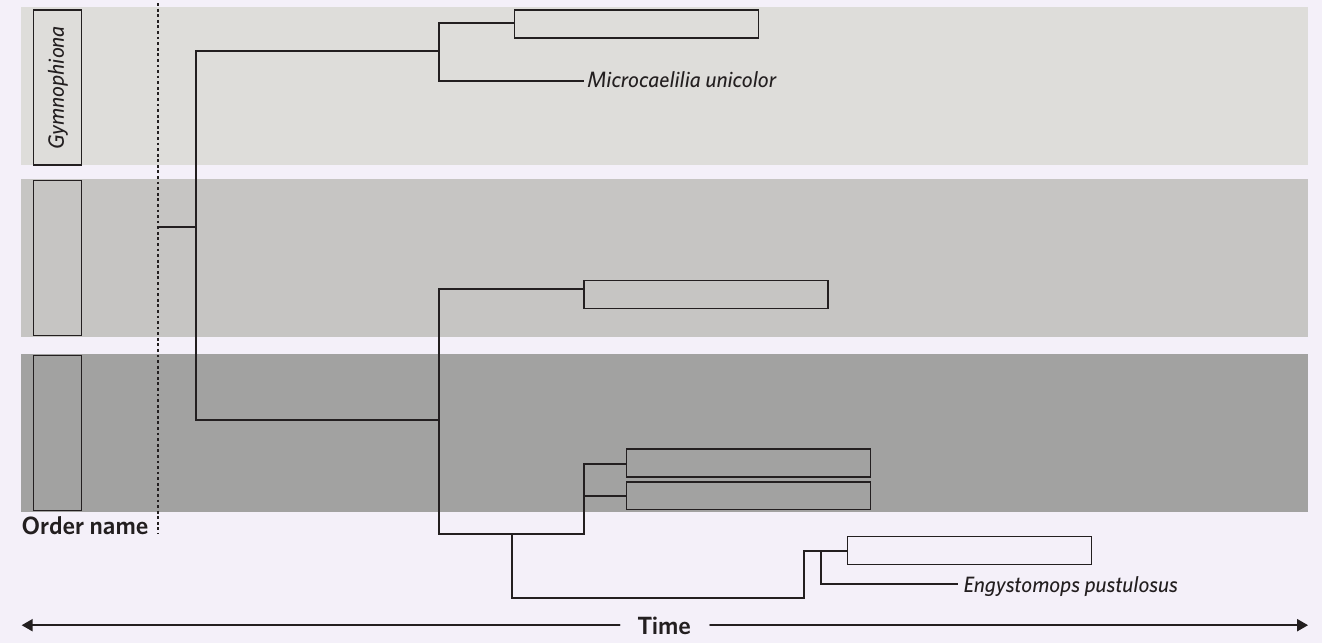
The phylogenetic tree shows evolutionary relationships through its branching pattern. Understanding how to read this tree is essential for answering questions about species relatedness.

Finding ancestor-descendant relationships: In some cases, the tree may show a direct line from one species to another, indicating a potential ancestor-descendant relationship. However, most phylogenetic trees show sister species (species that share a common ancestor but neither is the direct ancestor of the other).

Comparing relatedness between groups: To determine if one group is more closely related to a second group or a third group, trace back to find the most recent common ancestor. The group requiring fewer nodes to trace back is more closely related.

Working with genomic calculations

Understanding the complementary nature of DNA base pairing allows you to calculate missing information. Since guanine always pairs with cytosine, and adenine always pairs with thymine, the percentages must balance:

• If GC content = $44\%$, then AT content = $56\%$
• If you need to find thymine-adenine content, simply subtract the GC content from $100\%$

When working with genome assembly lengths, remember the conversion factor: 1 Mb = 1,000,000 nucleotides. This allows you to convert between megabases and individual nucleotide counts.

Key concepts for analysis

Understanding AT content: To find which species has the highest thymine-adenine content, look for the species with the lowest GC content (since GC + AT = $100\%$). Xenopus laevis has the lowest GC content at $39.35\%$, meaning it has the highest AT content at 60.65%.

Assessing taxonomic relatedness: When comparing how closely related different families are, use the phylogenetic tree structure. Families within the same order will be more closely related to each other than to families in different orders.

Exam tips

When answering phylogeny questions in exams:

• Always refer to the tree structure when determining relatedness
• Show your working when calculating nucleotide content or genome sizes
• Remember that closer branching points indicate more recent common ancestors
• Use the time axis to determine which species evolved first
• Consider all three orders of amphibians when making comparisons